Module 7 - Incorporating the Interrogator Unit
Introduction
This is a modular manual element that is used in the OS6 Administrator’s Manual, FAT Manual and Installer’s Manual.
It can be used for:
- Identifying and preparing an IU for deployment
- Replacing a faulty IU
- Fully commissioning an IU from scratch
Depending on the nature of the activity being considered some or all this manual may be required.
The manual is presented in the typical order required for a full set up from new of an IU, if an IU is being replaced into an existing configuration, users should take care with any setup that is being modified related to the configuration.
For example, if a fiber length is already known and used, exploiting the auto length detection routines may adversely affect the existing config and it is advised to stick with the existing configuration length.
Prior to using this manual, the user should be familiar with all IU maintenance aspects covered in the relevant product User Manual.
The user will also require the individual Interrogator Unit User Manuals for full detail on deploying and maintaining an Interrogator Unit
Laser Radiation Safety Notes
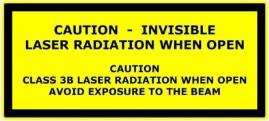
OptaSense® Interrogator Units (IU) includes laser products, these are classified in accordance with 21 CFR 1040.10 and IEC 608251. Please note the warnings in this document and attached to the unit, reproduced below – a typical example is shown below.
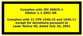


Use of controls or adjustments or performance of procedures other than those specified herein may result in hazardous radiation exposure.
In normal operation, the light emitted by an OptaSense® IU is completely contained within an optical fiber. The user must ensure appropriate controls (for example those described in IEC 608252) are in place to prevent unauthorised personnel breaking the continuity of the fiber, causing emission of invisible laser radiation.
Always switch off Laser Enable Keyswitch and remove the key before disconnecting or breaking the continuity of the fiber.
Do not operate an OptaSense® IU without an optical fiber connected.
Prior to connecting fiber always clean and inspect the connectors.
Consult an OTDR reading on a new connection prior to turning on and ensure that the behaviour is in line with the OptaSense Fiber Acceptance Specification OLA/329
Before turning on laser after a new fiber connection ensure that detectors are set to a maximum and follow the laser attenuation procedure detailed in this manual.
Consult the relevant Interrogator Unit User Manual for operations and maintenance activities.
For all installations the primary recommendation for fiber connectivity to an OptaSense® IU is a direct splice into the fiber. A secondary recommendation where a direct splice cannot be made is to use an (OptaSense® approved) APC connector to connect to the fiber. Use of any connectors not approved by OptaSense® is done so at the client’s own risk, which may cause significant damage to the IU, would invalidate any warranty and may result in a loss of system performance. Additionally, if an E2000/APC connector is used, the patch lead that connects the IU to the connector needs to be 30 metres long.
The lightning flash with the arrowhead symbol within an equilateral triangle is intended to alert the user to the presence of un-insulated ‘dangerous voltage’ within the product’s enclosure that may be of sufficient magnitude to constitute a risk of electric shock to persons.
Care must be taken whilst handling any of the equipment described in this manual. If any equipment is suspected to having been poorly handled, it must not be used before an adequate inspection can be made and continued safe operation verified.
Introduction to the OptaSense Family of Interrogator Unit
The Interrogator Unit (IU) is a core piece of equipment in the OptaSense® system. It probes the fibre and delivers measurement data to the Processing Hardware.
Most devices used in the OptaSense OS6 software are the OLA2.1(+) series of interrogators, however other units may also be encountered:
- OLA2.1(+) - The current “standard” Intensity only Interrogator Unit
- OLA2.2 – An Intensity only Interrogator Unit which can connect to two separate fibers using single laser. Both fibres will be displayed on the Backscatter plot simultaneously, as the IU has a single laser monitoring both fibers
- ODH-F – A quantitative IU that builds on prior OptaSense Interrogator Unit developments. Can also operate in a similar mode to the OLA2.1 units and is intended to be able to flexibly deliver similar performance levels to our OLA 2.1 although it is NOT intended to replicate it.
- QuantX - The QuantX system has been developed specifically to address sensing applications which require high quality quantitative phase and amplitude output and the practical levels of asset coverage whch were previously only available with a qualitative distributed acoustic sensing solution or over short ranges.
Further information on the Interrogator Unit (IU) can be found in the OptaSense System Specification, datasheet and the Interrogator Unit User Manual.
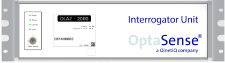
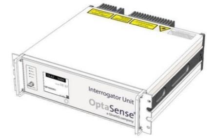
Figure 1: The front panel and isometric view of a typical OLA2.1(+) device.
Installing the Interrogator Unit
For all installation and use information please consult the individual Interrogator Unit User Manuals. Failure to follow these instructions may invalidate your warranty.**
Connecting to the Sensing Fiber
Preparation of Near End of Fiber
The IU is fitted with an E2000-APC female receptacle on the rear of the unit. The preferred method of connecting to a fiber is by splicing an E2000-APC pig tail or patch cable directly on to the sensing fiber and inserting into the rear of the IU.
Where a direct splice cannot be made and a patch panel is to be used, it is recommended to connect with a minimum 30m patch cable between the IU and the patch panel. The connections on the patch panel should also be of an APC variety.
Use of any connectors not approved by OptaSense is done at the client’s own risk, which may cause significant damage to the IU, would invalidate any warranty and may result in a loss of system performance. Contact OptaSense prior to any fibers being attached to the system and the IU’s laser being switched on. The OTDR traces must be supplied to OptaSense once the Termination Units and E2000/APC connectors have been attached.
It is important that before connecting to any new or unfamiliar fibers, an OTDR trace is measured to assess the conditions of the fiber and ensure that there are no significant reflections over the fiber.
Please ensure that all connected fibers match the requirements of OptaSense Fiber Acceptance Specification (OLA/329) prior to connecting.**
- Prior to connecting fiber ensure that the laser enable key switch is in the OFF position, attenuators are set to maximum and the key is removed.
- For optimum performance and particularly for short fiber lengths (<10 km) it is recommended that an OptaSense termination unit is fitted to ensure there is no end reflection.
- DO NOT insert a dirty or damaged optical fiber connector into the IU as this may contaminate or damage the internal connector.
- The OptaSense IU is fitted with a fully enclosed E2000-APC type connector which does not need service cleaning during normal operation.
- Direct splicing of the sensing cable into a patch panel is the preferred arrangement; however, should a splice connection not be possible, connection via APC patch cords may be used, each of which MUST be at least 30m length.
Verifying the End Condition with a Fiber Scope
The fiber scope must be used to check the cleanliness of any IU E2000 connector or E2000 patch cord connector. This task must be performed before connection any IU to any fiber even if the IU has come directly from the manufacturer.
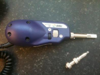
Figure 2: USB Fiber Scope
Before using the fiber scope the following is needed:
- The fiber scope.
- A laptop with “FiberCheck 2” installed this can be found on the disc located with the fiber scope or on your field engineers HDD. To install FiberCheck insert the disc and follow the on-screen instructions.
There are two types of connector to be used to check the patch leads and the IU E2000 connectors

Figure 3: ( left) Patch Lead Connector and (right) E2000 Connector
Once the right connector has been screwed onto the fiber scope the connector can then be tested.
Attach the fiber scope to a laptop via a USB port and start the FiberCheck 2 software. Ensure that the fiber type is set to single mode (SM) (See Figure 4 below)
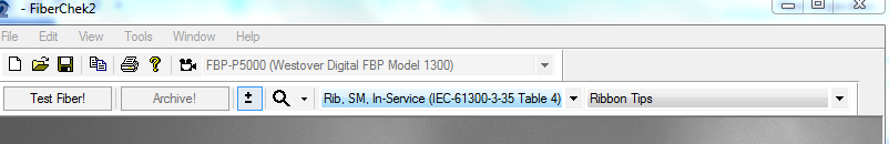
Figure 4: Fiber Type Selection
Push the fiberscope onto the E2000 patch lead connector or E2000 IU connector.
Push the small button located next to the focus wheel on the fiberscope to activate the camera. Confirm that an image comes up in the FiberChek2 software.
Use the focus wheel to bring the connector in to focus and once the percentage in the bottom right hand corner goes above 35% press the “Test Fiber” button on the software to take a picture of the fiber core.
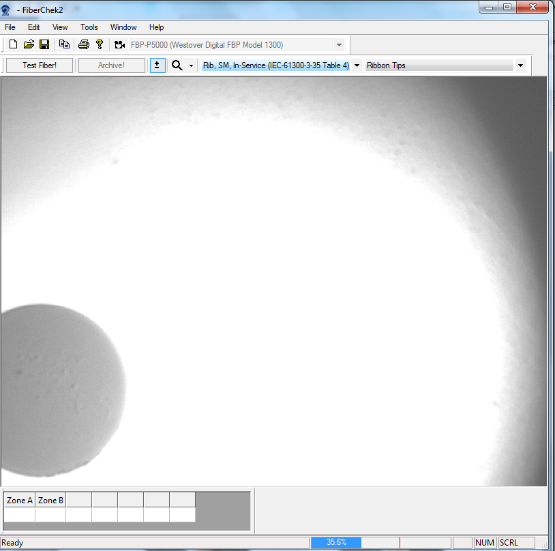
Figure 5: FiberCheck Software
The FiberCheck software will then process the image and return a pass or fail.
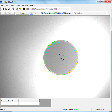
Figure 6 : FiberCheck Pass or Fail
If a pass is achieved the fiber end is ready to be used. If a fail is achieved, then the Fujikura One click should be used to clean the connector and the process should be followed again to check the fiber.
An image of the condition should be saved to verify that the system was correct on inspection.
NOTE: If the fiber check continually fails do not use the IU or patch cord. These items should be isolated and given to the engineer running the FAT to ensure that further testing/cleaning is carried out and as a last resort sent back to the manufacturer for replacement or repair.
Preparation of Far End with OptaSense Termination Unit
The fiber termination unit is a bespoke OptaSense development designed to eliminate reflections from the end of fiber termination. It should be spliced on to the end of the sensing cable to suppress end reflections.
The marked unit can be placed inside the patch panel and needs no further treatment.
| Specification | OptaSense single mode termination unit |
|---|---|
| Length | 150mm |
| Connection Type | Fiber pigtail (direct splice) |
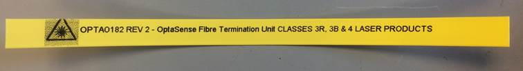
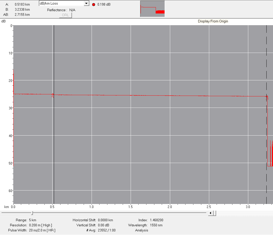
Figure 7: Fiber termination unit and end suppression evident on OTDR trace – no end of fiber return spike that would appear with a conventional splice
Making the Final Fiber Connection
All the fiber connectors once cleaned can be connected using the methodology appropriate to the specific connectors. In the case of the OptaSense E2000 connectors, the connector block should be guided into the matching receptacle on the rear of the IU and pushed home until a positive click is heard / felt. Some modest resistance may be experienced, and this will need to be overcome until the connection fully latches home.
To connect the fiber, remove the protective dust-cap by simply pulling the tab to withdraw it. Insert the connector immediately and check that it clicks into position. When removing the fiber, replace the dust cap immediately to prevent contamination of the IU output connector.
Do not operate the IU without an optical fiber connected. Following the procedures in this manual and taught during training will ensure that the laser is only switched on when safe to do so.
Only disconnect or break the continuity of the optical fiber with the Laser Enable Keyswitch turned to the off position (the Laser Enable LED will be off) and the key removed.
Preparing an OptaSense OLA2.1(+)/OLA2.2 IU For Service
The majority of OS6 installs will use OLA2.1(+) IUs. For all models within the 2.1/2.2 range the setup instructions use the same software interface and is covered in detail below.
Consult the IU specific manuals for further information on the setup for an ODH-F and QuantX units.
The process for setting up the lasers follows a few discrete steps:
- Changing the IP address of the IU (if required)
- Set the fiber length, sample rate, resolution and verify position of end of fiber
- Verify that there are no reflections present in the fiber which could cause damage to the system or degradation of signal
- Optimise power density of the signal present in the fiber (achieving maximum signal to noise ratio, whilst ensuring the system is operating in a linear manner, i.e. too great a power density (low launch attenuation) will deliver non-linear performance and incorrect results. The non-linear point can be easily be identified in longer fibers (>10km) but in short fibers we need to establish the correct attenuator settings slightly differently.
- Manually verify the auto attenuation settings
- Verify that the start of the fiber (back of IU box) is set to channel zero.
- Configure fiber break if required. The OLA2.1+/OLA2.2 and QuantX IUs make use of an IU assurance stream and have a self-configuring fibre break detector.
Before switching on the laser for the first time it is vital to ensure that the IU is in a safe state. This is achieved by setting both the launch and detect attenuators to maximum (approximately 27dB).
Identifying the IP Address of the IU
Please refer to the OptaSense supplied network diagrams for system information and IP addresses.
There are two separate procedures for connecting a new IU. The procedure taken is dependent on whether the IP address of the replacement IU is known or unknown. On the newer OLA2.1(+) and ODH-F IUs the IP address is displayed on the E-ink screen on the face of the IU.
IUs without an E-ink Display
To change the IP address of an IU with an unknown IP address:
-
Connect a laptop or a PC directly to the IU with an Ethernet Cable using Ethernet Port 1 on the IU.
-
Use IP locating software such as NMap or Wireshark to retrieve the IP address of the IU if the IP address is unknown. Make sure that the IP address of the laptop is as close so the suspected IP address of the IU as possible. The manufacturing default for the IU is 192.168.0.33. The address range is typically 192.168.XXX.XXX.
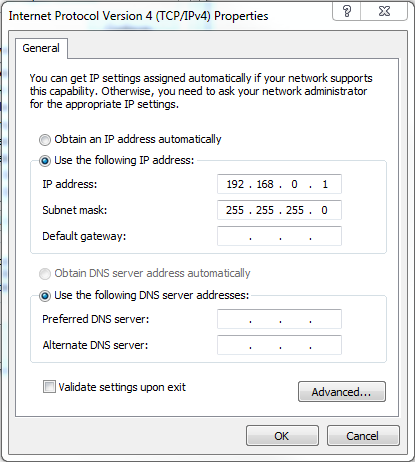
Figure 8: Changing the IP address and Subnet mask of the connected laptop
-
Once the IP locating software has verified the IP address of the IU the standalone version of the IU setup tool can be run to change the IP address of the connected IU. The IP address of the laptop running this tool must be changed to allow connection to the IU’s existing IP address (Figure 8).
IUs with an E-ink Display
The IP address of an OLA 2.1 can simply be read from the front panel (even whilst off). If the IU is turned on and displaying a different page, press the marked button to cycle through the information pages until it returns to the main information display.
Making an Initial Connection
Once you have confirmed the IU IP address and verified that you can communicate to it (e.g. by ping) then the IP address can be changed to the desired value.
For an IU that is being replaced or setup to a different sub net than that allowed on the actual configured system you may need to first change this externally, e.g. in a stand-alone laptop deployment.
Changing the IP address of an IU can be completed through the OS6 IU Setup tool, accessed via the configure drop down menu or by typing IU Setup in the global search (Figure 9). Open the IU setup, on the left-hand side of the OLA IU Setup main window (Figure 10) select the OPS of the IU you require to change the IP address.
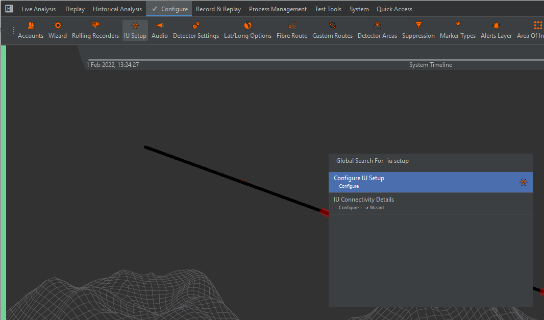
Figure 9: IU Setup via Configure Menu and IU Setup via global searc
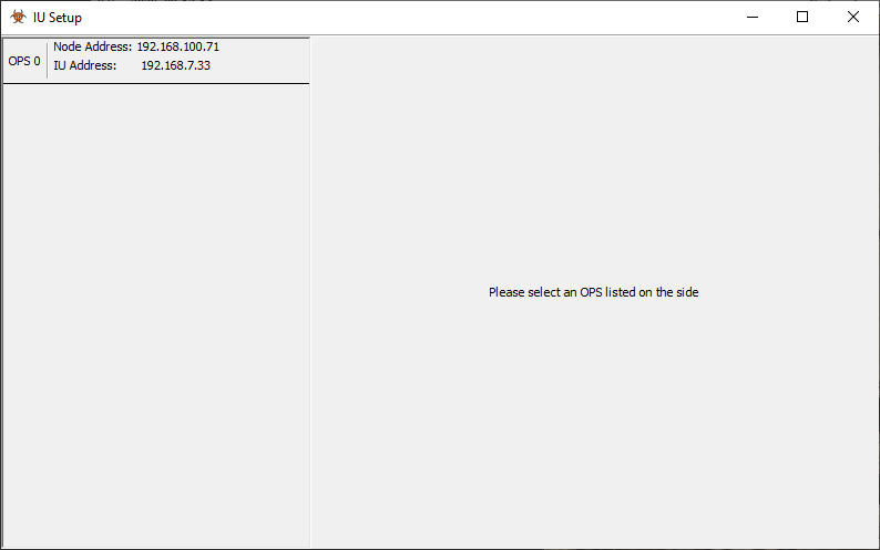
Figure 10: OS6 IU Setup main window
On first running its unlikely that the IU will have the IP address specified in your config, in this instance, you will need to go to the Wizard and select IU Connectivity Details (Figure 11) to change either the type of the connection (OLA 2.1 / ODH-F / QuantX) and/or the IP address desired to connect to.
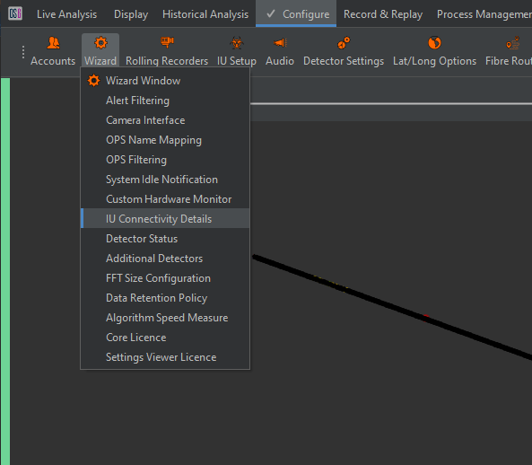
Figure 11: Change IU connection
A window will then appear (Figure 12) where you can select the interface type and/or change the target IP address.
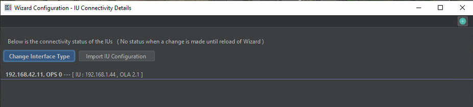
Figure 12: Change IU Connection / Interface Type
Changing the Address of the connected IU
Once the IU setup has connected to the IU (Figure 13) the right window pane will be populated, and the ‘Connect’ button will be shown in green. To change the IP address, select the Edit button to the right of the IP.
Note: All screen shots here are for an OLA2.1(+).
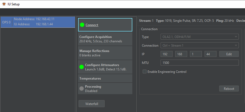
Figure 13: IU Connect Window
This brings up the Change IP Address window (Figure 14), enter the required IP address from the ND and ‘press OK’. It is then required to power cycle the IU. Once power has returned it is possible to check the IP address has changed on the front of the IU.

Figure 14: IU IP address Window
At this point you can either transfer the connection back to the processor using a stand-alone or continue, you may need to change the subnet IP address of your connected device.
Setting the IU into a safe condition before turning on the laser
The interrogator is fitted with two attenuators which act to decrease available length:
- Launch attenuator – decreases the amount of available light. Can be used to limit the light in a long fiber and ensure that operations are within the linear regime
- Detect attenuator – used to modulate the overall value in any deployment to ensure it is not limiting or clipping at the detector
Prior to setting the attenuators for the IU, the Interrogator must be placed into a SAFE mode to avoid damage.
To do this, select the Configure Attenuators. For an OLA2.1(+)/OLA2.2 set the Launch and Detect to approximately 27dB.
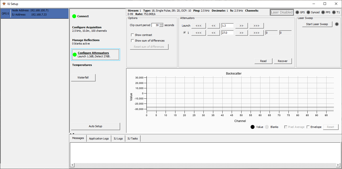
Figure 15: Configure Attenuators Display
To increase the Launch and Detect attenuators use the ‘>>’ buttons to increase the attenuation. The ‘>>>’ icon will increase attenuation by a greater amount. The ‘<<<’ and ‘<<’ buttons will reduce the amount of attenuation.
Once the attenuators have both been and the fiber has been checked to confirm no large reflections using an OTDR, the laser can be switched on at the IU (both front and back panels for OLA 2.1+/2.2)
Auto Setup Function
When the IU is connected the user can proceed to setup the IU using the Auto Setup tab.
If you are using this with a pre-existing configuration, this section should be performed to check that the acquisition parameters required by the config are being replicated by the IU. They should be picked up by the config and passed to the IU, however there is no harm in preparing the IU with the expected values in advance.
For complex situations it is advisable to replicate these first before connecting to the config. Similarly, in all situations the Auto Setup results should be checked.
The Auto Setup function has been designed to acquire all the parameters needed for the successful setup of the IU. Requirements such as Data Type, Ping Rat as well as laser Launch and Detect values will all be determined (Figure 16).

Figure 16: Auto Setup function
Wen the Auto Setup button is actioned, the operator will be presented with the following dialog
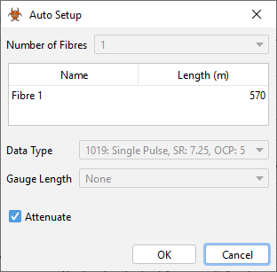
Figure 17: Auto Setup dialog
The operator is expected to to enter the fibre length in metres. This information should be known, if not the customer should have this information.
For OLA2.1(+) the number of fibres cannot be changed and is set to ‘1’
For OLA2.2 a maximum of two fibres can be connected to this IU. If this is the case, select ‘2’ fibres and enter the two fiber lengths.
In all cases the Auto Setup will select the ‘best’ Sample Rate and Data Type for the entered Fibre Length.
When the Auto Setup is running, a pulsing notifier will be present on the “Auto Setup” button which turns into an “Abort Auto Setup” button.

Figure 18: Appearance during Auto Tune
The Auto Setup function appears at each display within the IU setup. It will carry out the same function irrespective of which display the user is observing.
It is important to monitor the Auto Setup process, paying attention to the status box on the right side of the screen. Unlike the previous Auto Attenuate function, the Auto Setup function now incorporates all the previous auto functions and will now take longer to fully complete.
Once the Auto Setup function has been started the IU firstly increases the detect attenuator to its maximum value, it then changes the launch attenuator value and sweeps through all the launch values until it detects clipping. It then monitors for clipping over a 30 second period to ensure that only a modest amount of clipping occurs.
It will then establish the fiber length and use this information to determine the most appropriate Data Type and Ping Rate.
Auto Setup will then carry out another attenuation of the laser, adjusting the launch and detect settings accordingly.
It is recommended that after Auto Setup has been run the operator zooms into the last 200 channels and adjusts the launch attenuator to check the non-linearity point.
The Auto Setup tool is provided as an aide but should be verified by a competent, trained individual.
When the Auto Setup has completed and the final launch and detect attenuators have been set it is recommended that you monitor the Detector Clipping (Figure 21) to ensure that the IU is not clipping above specification, specifically at the start of the fiber near to the IU itself as this can damage the detect sensor. If an IU is clipping too much, then the traffic light will turn Red and emit ADC Clipping errors to the user. An amount of clipping is always to be expected and is normal. The detector statistics are monitored by the system.
When the detector clips excessively it will send an error to the GUI. Clipping will appear as a statistical variation; this does not imply there is a problem and can indeed be a positive indication that the IU is using maximum dynamic range. Where this becomes an issue is when clipping errors appear continuously, this indicates a serious problem that should be addressed.
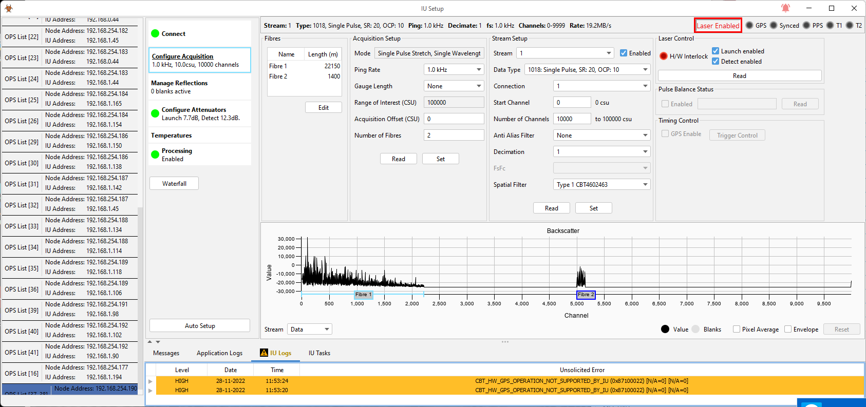
Figure 19: OLA2.2 Backscatter plot – 2 fibers/single laser
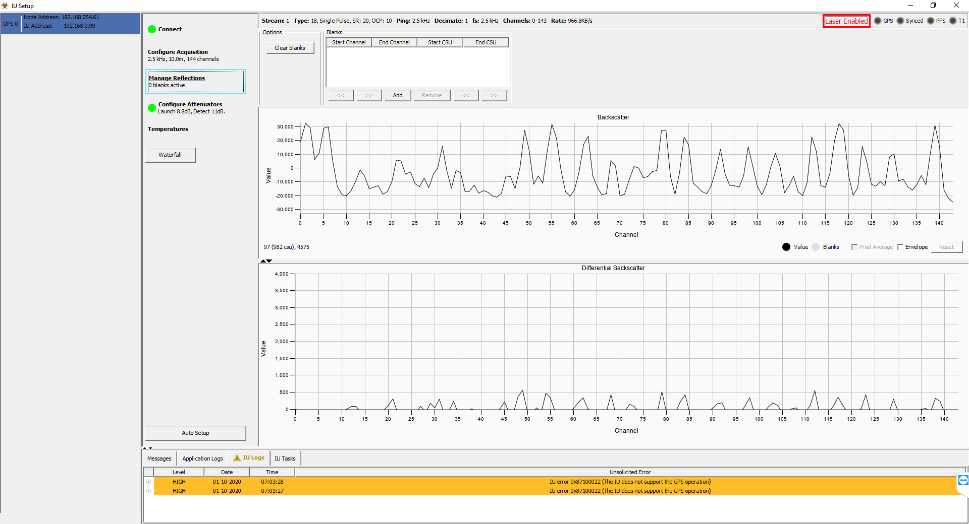
Figure 20: Manage Reflections Display
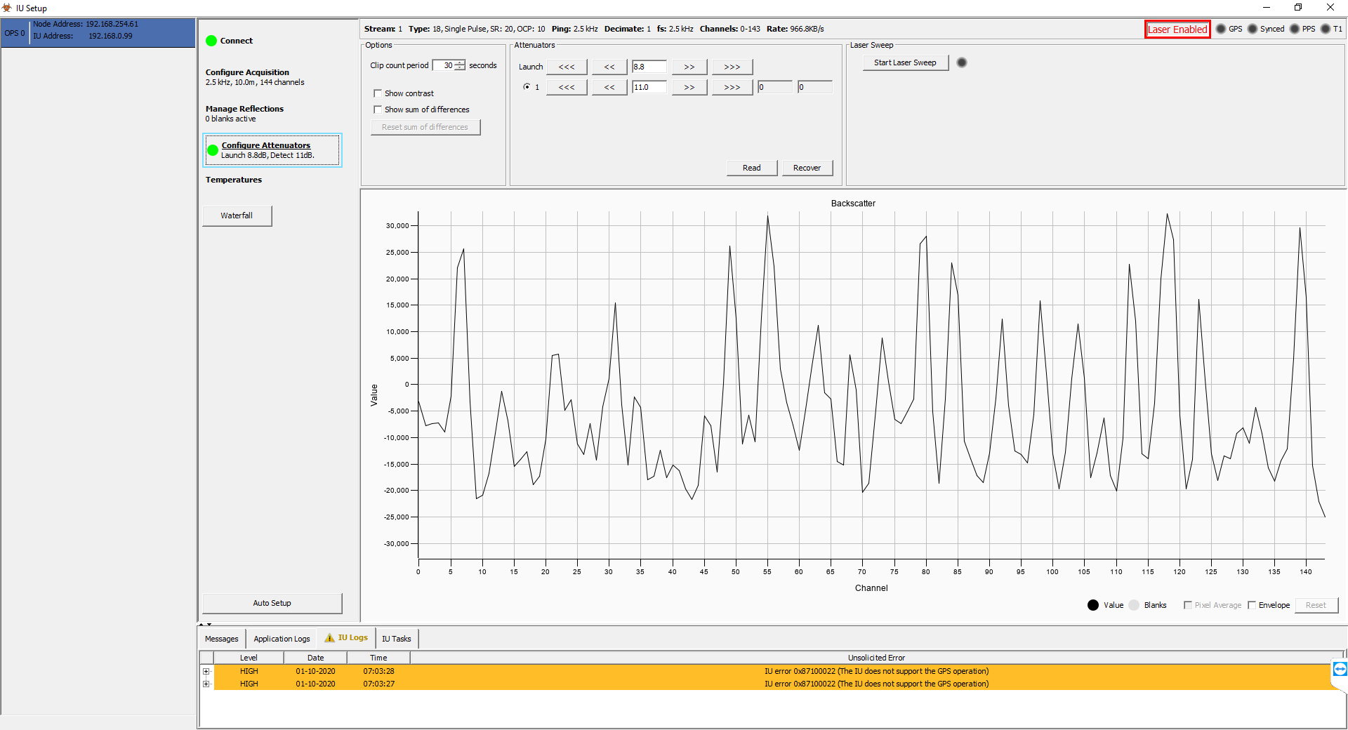
Figure 21: Configure Attenuators Display
Additional Setup Functions
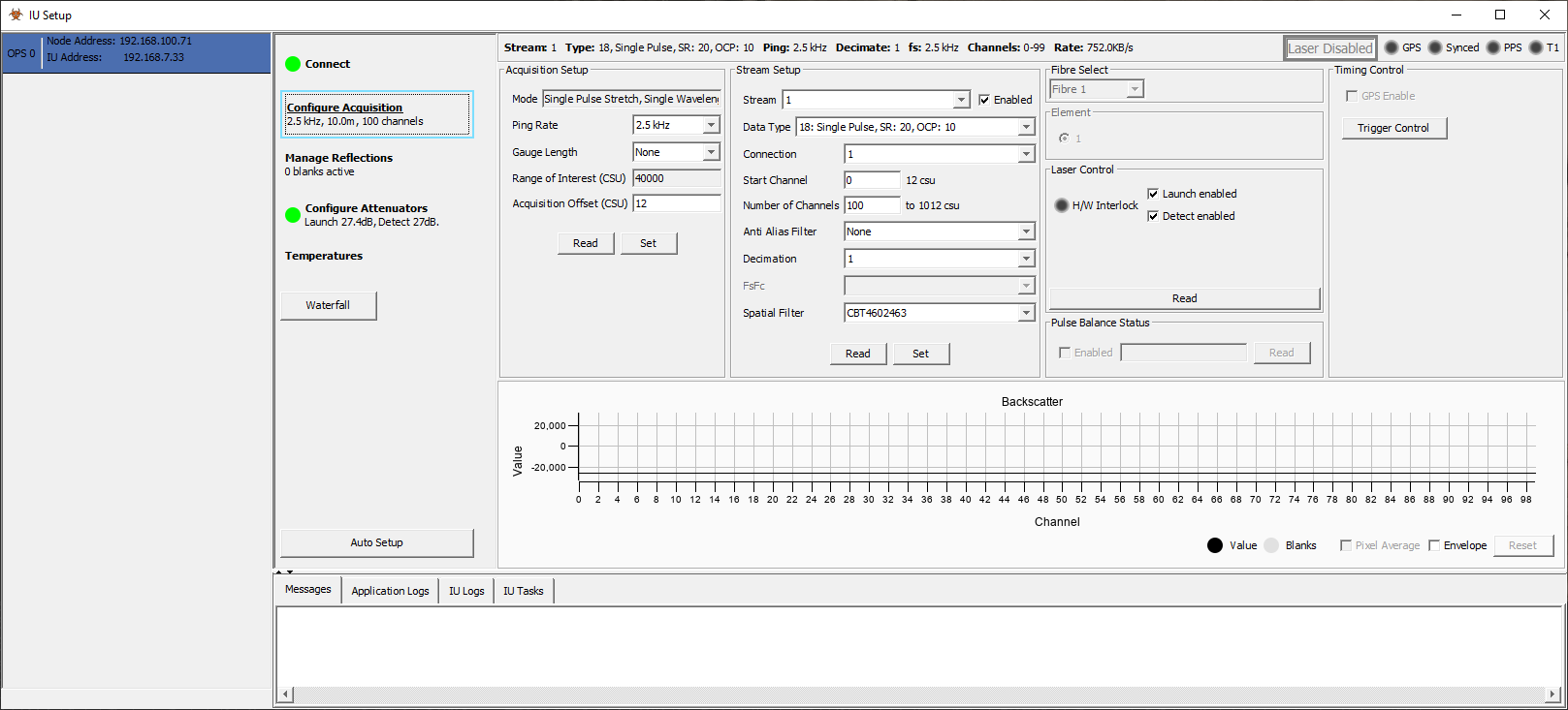
Figure 22: Configure Acquisition Display
Options for fiber length, sample rate and spatial resolution
If a sensing fiber that is connected is LONGER than the stated fiber length (i.e. crossover approach), the settings will need to be saved as they are not maintained on reboot of the IU.
In normal circumstances there is only a single fiber length to consider – the physical length of the fiber is equal to the sensing length. This, together with the channel size defines how many channels the system will operate with.
Additionally, the sample rate reduces with increasing fiber length. This is a matter of simple physics; we cannot send a new laser pulse down the fiber until the scatter from the end of the fiber has reached the detector.
In the circumstances where we are operating with a fiber length longer than the sensing length, the following rules should be noted:
- Fiber Length should be set to the sensing length (the crossover point)
- Channel size should be set commensurate with the fiber length
- Sample Rate should be set commensurate with the full physical fiber length
In all cases the results of the process should be compared to the results of an OTDR and to expectation – the Auto Setup function is provided as an aide but should always be verified by a competent, trained individual.
Stream Setup – Decimation
OptaSense IUs can output decimated data streams for certain data types. If a selected decimation factor is not supported for the combination of IU & Data types then it will be rejected. Software provided decimation can be applied from the ‘Processing’ Tab (see Section 8.6).
Verifying the settings – OLA2.1(+)/OLA2.2
- The Auto Setup option can be used to attenuate lasers as well as establishing the fiber length although the fiber length should always be confirmed using an OTDR. The setup process may take a couple of minutes and the status can be seen in the Status output. However, the results from the Auto Setup feature should be verified manually. See the manual steps below.
- During the Auto Setup procedure, the IU first increases the detect attenuator to its maximum value, it then changes the launch attenuator value and sweeps through all of the launch values until it detects clipping. It then monitors for clipping over a 30 second period to ensure that no clipping occurs.
- After the process is completed, it is recommended that the user zooms into the last 200 channels of the fiber, decreases the launch attenuator and verify that the non-linearity point occurs. Note that non-linearity points should not occur for short fibers (less than 10 km) and in these cases this step can be skipped.
- After Auto Setup is complete, the user should observe for Detector Clipping especially at the beginning of the fiber. If significant clipping occurs then the detect attenuator should be increased until this no longer occurs.
Preparing an OptaSense ODH-F IU For Service
ODH-F builds on prior OptaSense Interrogator Unit developments and is intended to be able to flexibly deliver short-range (<15 km) quantitative data or long range qualitative data with similar performance levels to our OLA 2.1 although is NOT intended to replicate it.
There are 4 variants of the ODH-F, an intensity only variant (Base model, CBT4800000 Basic), a multiplexing intensity only variant that allows the acoustic intensity of up to 4 cables to be monitored (4 Way Multiplexer, CBT4800000 MUX), a quantitative variant capable of doing everything the base model is capable but also of acquiring quantitative data (Quantitative Phase and Amplitude model, CBT4800000 Quant) and a multiplexing quantitative variant (4 way Multiplexer AND Quantitative Phase and Amplitude model CBT 4800000 MuxQuant) that allows the interrogation of 4 cables and acquisition of quantitative data.
Many of the configuration practices are similar or the same as for the previously mentioned IU’s. The configuration procedure to use is dependent on how the IU is being used (amplitude only or quantitative mode, with or without multiplexing). This guide discusses the configuration required for all these operation modes, dependent on the unit not all these modes may be accessible. Connection to the IU and data types are also discussed.
OS6 does not at the current release support Multiplexing in ODH-F.
Connection to the IU
Ensure that the laser key is switched off and there is no light being transmitted into the fiber. To connect to the IU, open the IU setup page in the engineering tab. Select the appropriate OPS from the IU setup page. If the IU IP address has already been setup this will connect, if not then the loading will time out and the IU connection will need changing.
Change the IP address and interface type in the popup box in the same way as for the OLA 2.1(+). As with the OLA 2.1(+) the ODH-F units IP address is displayed on the e-ink display when the unit is powered down. The default for this is 192.168.0.40. The interface type should be “ODH-F”. Once edited, select update.
Data types
A range of non-quantitative and quantitative data types are available in the ODH-F:
| Type | Description | Type |
|---|---|---|
| 1001 | Single Pulse SR 1.5 OCP 1 | Non-quantitative |
| 1002 | Scope Data | Quantitative |
| 1003 | Launch Pulse Diagnostic Data | Non-quantitative |
| 1004 | Diversity Stacked OCP 8 | Quantitative |
| 1005 | Diversity Stacked Metadata OCP 8 | Quantitative |
| 1009 | Phase OCP 1 | Quantitative |
| 1012 | Dual Pulse ADC OCP1 | Quantitative |
| 1013 | Diversity Stacked DC OCP 8 | Quantitative |
| 1014 | Diversity Stacked Metadata DC OCP 8 | Quantitative |
| 1015 | Single Pulse SR 1.5 OCP 8 | Non-quantitative |
| 1018 | Single Pulse SR 20 OCP 10 | Non-quantitative |
| 1019 | Single Pulse SR 7.25 OCP 5 | Non-quantitative |
| 1024 | Phase OCP 1 0.001xfs cutoff | Quantitative |
| 1061 | Scope Data Max | Non-quantitative |
| 1062 | Single Pulse SR 1.5 OCP 1 HdB | Non-quantitative |
| 1063 | Single Pulse SR 1.5 OCP 8 HdB | Non-quantitative |
| 1064 | Single Pulse SR 20 OCP 10 HdB | Non-quantitative |
| 1065 | Single Pulse SR 7.25 OCP 5 HdB | Non-quantitative |
OCP= Output Channel Pitch, SR= Spatial resolution.
The best data type to use is dependent on the application. Quantitative data can only be collected from shorter length cables (<15km), so this limits the applications that can have quantitative data collected. As such for applications requiring the monitoring of longer assets, non-quantitative data must be collected. Quantitative data has the advantage that it collects phase information about the acoustic waves interacting with the cable, allowing more detailed/ accurate analysis of the data.
In terms of the non-quantitative data types the significant difference between each type is the OCP and SR lengths of the data type. The optimum spatial resolution is a function of the required sensitivity (the larger the gauge the lower the signal to noise ratio) and the frequency content of signals to be detected (the higher the frequency needing to be monitored the shorter the gauge length should be, due to spatial averaging). Data type 1018 is an equivalent to the 20m gauge of the OLA 2.1.
The main quantitative data types are DT1004 and DT1013. Data type 1004 is diversity stacked quantitative data with a high pass filter to remove low frequency signals. Data type 1013 is equivalent to DT1004 with the high pass filter removed in the signal processing chain. Both of these have an OCP of 8 m. In most situations the low frequency content is informative and data type 1013 should be recorded. DT1009 provides quantitative phase data with no diversity stacking and an OCP of 1m. This datatype is oversampled spatially. A heavily decimated version of DT1009 is available as DT1024, which can be used for recording very low frequency measurements.
Data type 1002 is the scope mode for the dual pulse configuration that gives the optical amplitude for reflected light and is used to setup the launch and receive attenuators for collection of quantitative data.
Non-Quantitative data acquisition setup
The configuration of the ODH-F for collection of non-quantitative data is the same as for the manual configuration of the OLA 2.1. At present the auto configuration feature will not work with the ODH-F. Start with the laser interlock key turned to the off position and set both launch and detect attenuators to > 24dB. To configure the ODHF for non-quantitative data the appropriate data type, number of channels, first channel to acquire and ping rate are selected in the same way as for the OLA 2.1. The attenuators are configured in the same way as the manual configuration of the attenuator setting for the OLA 2.1 (see section 8.1) using DT1002.
Quantitative data acquisition setup
To configure the ODH-F for collection of quantitative data start with the laser interlock key turned to the off position and set both launch and detect attenuators to > 24dB. DT1002 needs to be selected prior to carrying out the manual tuning of the attenuators (see section 8.1). A decimation factor of 4 should be set for quantitative data. The number of channels, first channel to acquire, and ping rate should also be set appropriately for the specific fiber under investigation (use the OTDR length for this). Once the attenuators are configured the data type can be set to whichever quantitative data type is suited best to the measurement.
Stream Setup – Decimation
OptaSense IUs can output decimated data streams for certain data types. If a selected decimation factor is not supported for the combination of IU & Data types then it will be rejected. Software provided decimation can be applied from the ‘Processing’ Tab (see Section 8.6).
Multiplexing
In an ODH-F with multiplexing capability up to 4 fibers can be monitored. At present the OS6 software does not support multiplexing.
Preparing an OptaSense QuantX IU For Service
The QuantX system has been developed specifically to address sensing applications which require high quality quantitative phase and amplitude output and the practical levels of asset coverage that were previously only available with a qualitative IUs solution.
It is important to note that prior to any operation of the QuantX, the transport bolts must be removed. Detailed information on this can be found in the IU User Manual.
Identifying the IP Address of the IU
Please refer to the OptaSense supplied network diagrams for system information and IP addresses.
If communications to the IU fail, then the IP address will need to be established. At this stage it is worth noting that the manufacturing default IP address is 192.168.0.30. Unlike the OptaSense OLA2.1(+) and ODH-F IU’s previously described, the QuantX IU has no screen on the front panel and therefore the existing IP address of the IU must first be established.
To establish the IP address of a QuantX IU the following steps should be taken:
-
Connect a laptop or a PC directly to the IU with an Ethernet Cable using Ethernet Port 1 on the IU.
-
Use IP locating software such as NMap or Wireshark to retrieve the IP address of the IU. Make sure that the IP address of the laptop is as close so the suspected IP address of the IU as possible. The manufacturing default for the IU is 192.168.0.30. The address range is typically 192.168.XXX.XXX.
Figure 23: Changing the IP address and Subnet mask of the connected laptop
- Once the IP locating software has verified the IP address of the IU the standalone version of the IU setup tool can be run to change the IP address of the connected IU. The IP address of the laptop running this tool must be changed to allow connection to the IU’s existing IP address.
Making an Initial Connection
Once you have confirmed the IU IP address and verified that you can communicate to it (e.g. by ping) then the IP address can be changed to the desired value.
For an IU that is being replaced or setup to a different sub net than that allowed on the actual configured system you may need to first change this externally, e.g. in a stand-alone laptop deployment.
Changing the IP address of an IU can be completed through the OS6 IU Setup tool, accessed via the configure drop down menu or by typing IU Setup in the global search (Figure 9). Open the IU setup, on the left-hand side of the OLA IU Setup main window select the OPS of the IU you require to change the IP address (Figure 10).
On first running its unlikely that the IU will have the IP address specified in your config, in this instance, you will need to go to the Wizard and select IU Connectivity Details to specify the IU type (QuantX) and/or change the IP address (Figure 11).
A window will then appear where you can select the interface type and/or the target IP address.
Changing the Address of the connected IU
Once the IU setup has connected to the IU (Figure 13) the right window pane will be populated, and a traffic light of connection will be shown in green. To change the IP address, select the Edit button to the right of the IP address (Figure 13).
This brings up the Change IP Address window (Figure 14), enter the required IP address from the supplied network diagram and ‘press OK’. The IU will then need to power cycle in order to enact the change.
At this point you can either transfer the connection back to the processor using a stand-alone or continue, you may need to change the subnet IP address of your connected device.
Setting the IU into a safe condition before turning on the laser
The interrogator is fitted with two attenuators:
- Launch attenuator – adjusts the amount of light launched into the fiber. Can be used to limit the light in a long fiber and ensure that operations are within the linear regime
- Detect attenuator – used to limit the amount of light received by the detector in order to protect the sensitive photodetectors
Prior to setting the attenuators for the IU, the Interrogator must be placed into a SAFE mode to avoid damage.
At this point it is worth nothing following the initial start-up of a QuantX unit, the detect attenuator will always revert to the SAFE position.
To set the QuantX IU to SAFE mode, select the Configure Attenuators tab (Figure 15). Set the Launch and Detect fields to approximately Launch: 20 dB and Detect: 40 dB.
To increase the Launch and Detect attenuators use the ‘>>’ buttons to increase the attenuation. The ‘>>>’ icon will increase attenuation by a greater amount. The ‘<<<’ and ‘<<’ buttons will reduce the amount of attenuation.
Once the attenuators have both been set to SAFE values (approximately 20 dB for Launch and 40 dBfor Detect) and the fiber has been checked to confirm there are no large reflections using an OTDR, the laser can be switched on at the IU.
Data types
The following data types are available for QuantX. Note where the data types refer to single or dual pulse, this should NOT be confused with being Quantitative and Non Quantitative modes, rather the pulses here are referred to the number of information carriers.
| Drop Down Option | Data Type | Description |
|---|---|---|
| ADC Data | 1074 1075 | ADC Data (single pulse) - Raw ADC Data for Engineering Use (not used) ADC Data (dual pulse) - Raw ADC Data for Engineering Use (not used) |
| Scope Data | 1076 1077 | X Y Scope Data (single pulse) – Used for Optical Optimisation X Y Scope Data (dual pulse) – Used for Optical Optimisation |
| Phase Data | 1078 1079 1080 1081 | Diversity Processed Phase (single pulse) – 1m OCP (10 CSU) Diversity Processed Phase (dual pulse) – 1m OCP (10 CSU) Diversity Processed Phase (single pulse) – 10m OCP (100 CSU) Diversity Processed Phase (dual pulse) – 10m OCP (100 CSU) |
The Data Type and Carrier Mode to be used is selected via the data type drop down. Once the Data Type is selected, it is important that the “Set” button is pressed to ensure the selected Data Type is being used.
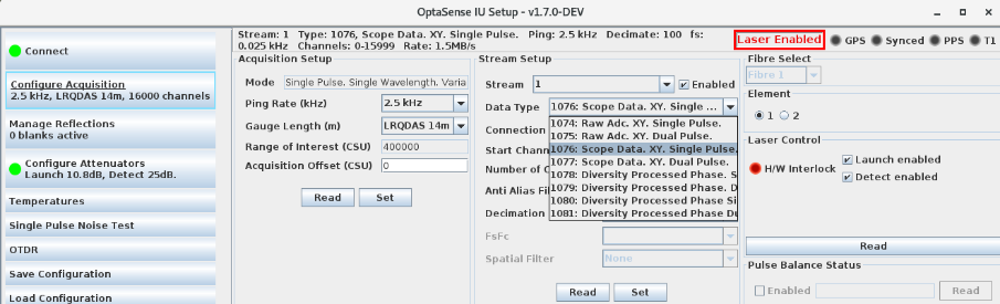
Figure 24: Selecting Data Type
Upon reconnection to a unit that has already been configured, these controls may not reflect the current settings. At any time, the “Read” button can be pressed to read the settings out of the IU and confirm the configuration. The status bar at the top of the screen always shows information about the data that is being received.
Choice of Mode of Operation (1- or 2- carrier)
The fundamental mode of operation is to launch a pulse of light into the optical fiber. The Rayleigh Backscatter returned to the IU is then analysed, allowing the time-varying phase signal from along the fiber to be determined.
The IU can operate in either “Single Carrier” (data types 1078 and 1080) or “Dual Carrier” mode (data types 1079 and 1081). In dual carrier mode, the IU uses two independent pulses to interrogate the fiber. This provides two overlaid, semi-independent backscatter patterns, each providing an independent measure of the phase data which can then be combined to reduce the effects of fading. While reducing fading, this can be detrimental to the data quality through the introduction of inter-carrier crosstalk (particularly where large signals are present) and a small general increase to the noise levels. Nonetheless, for some applications the benefits are likely to outweigh the drawbacks.
The optimum mode will depend on the specific situation and signals of interest:
Single Carrier Mode is best where:
• Large, high frequency, signals are present
• Spatial discrimination is important
• The fiber has low losses
• The loss / range profile sits well within the Performance Envelope
Two Carrier Mode is best where:
• Performance at long range is important
• Losses are challenging
• Longer gauge lengths are being used
Interrogation (Ping) Rate
The maximum interrogation (Ping) rate is determined by the length of the connected fiber. Best performance is obtained using the maximum rate possible for the fiber, with subsequent time-domain decimation if the band of interest is less than Ping Rate / 2.
The maximum interrogation Rate (kHz) for a fiber of length L (km) is determined by:
IRmax (kHz) = 100 / L (km)
For best performance, use the nearest Ping Rate from the drop down that is smaller than the calculated maximum from knowledge of the connected fiber length.
Note – if the selected and calculated rates are very close, inspect the backscatter closely at the beginning and end of the waterfall as different fibers will have slight differences in propagation velocity which may cause overlap. If the IU is pinging too fast for the fiber length, the backscatter signal from the end of the fiber will be superimposed on the start of the next interrogation cycle, producing interference/noise on the front end of the trace.
| Interrogation Rate | Nominal Acoustic Bandwidth | Max cable Length | QuantX | QuantX-LR |
|---|---|---|---|---|
| 0.5 kHz | 250 Hz | 160 km | ||
| 0.8 kHz | 400 Hz | 100 km | ||
| 1 kHz | 500 Hz | 80 km | ||
| 2 kHz | 1 kHz | 40 km | ||
| 2.5 kHz | 1.25 kHz | 40 km | ||
| 3.125 kHz | 1.56 kHz | 32 km | ||
| 4 kHz | 2 kHz | 25 km | ||
| 5 kHz | 2.5 kHz | 20 km | ||
| 8 kHz | 4 kHz | 12.5 km | ||
| 10 kHz | 5 kHz | 10 km |
Table 1: Key operating parameters for QuantX / QuantX-LR
Note that the Maximum Cable Length is that to which the IU may be connected – it does not imply data will be delivered – this is limited to 50km (5,000 10m OCP).
Stream Setup – Decimation
OptaSense IUs can output decimated data streams for certain data types. If a selected decimation factor is not supported for the combination of IU & Data types then it will be rejected. Software provided decimation can be applied from the ‘Processing’ Tab (see Section 8.6).
Managing Reflections and Fiber Breaks
An advanced feature of the IU Setup is the Manage Reflections section (Figure 25) this enables the user to blank out a number of channels where there is a reflection from an event down the fiber, such as a bad splice, micro bends, fiber breaks or the end of the fiber. It is recommended that the advanced manage reflections is only used if the fiber cannot be repaired or the fault removed.
You can attempt to manage the fiber break before repair by creating a single or multiple reflection blanking zones.
Navigate to the IU Setup and select the Manage Reflections tab (Figure 25). In the Blanks box press the Add button to create a new blank. This is the start process to adding your start and end channel values.
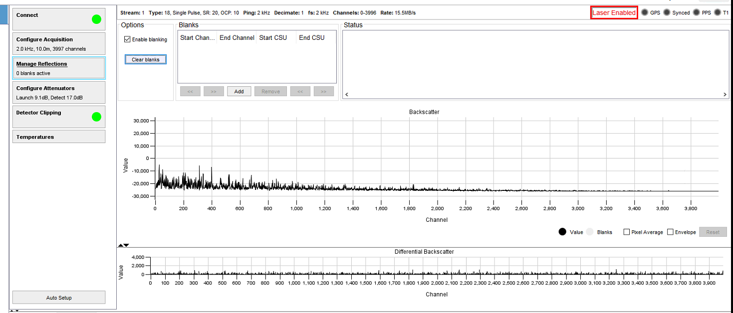
Figure 25: Manage Reflections tab in IU Setup
To identify the Start and End channels, adjust zoom to the start of the reflection event within the Backscatter panel, from this example the Start Channel is 1000. Double click the Start Channel cell and enter this value into the blanks box highlighted then Press enter (Figure 26).
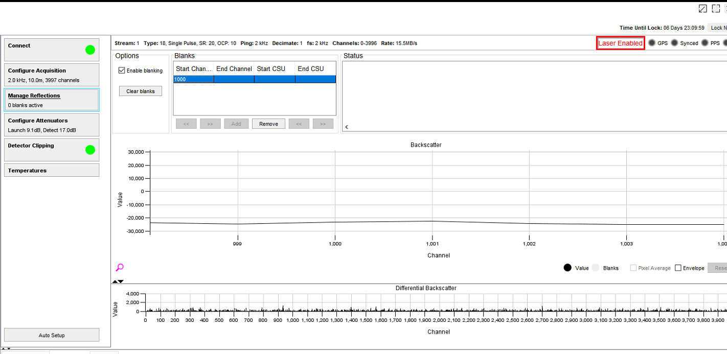
Figure 26: Start Channel cell & Backscatter Panel
For the end channel, locate the channel in the backscatter panel as before and double click the End Cell to enter the value (Figure 27). The blank that is being applied will normally only be a few channels but to assist with the visual representation the blanks applied here are much larger.
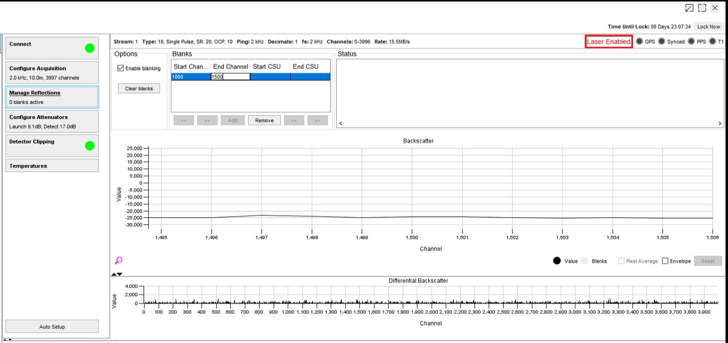
Figure 27: End Channel Cell & Backscatter Panel
As you can see highlighted in the backscatter panel the blanking zone has been created. The added blanking zone is shaded on the backscatter panel to provide visual indication of the region it covers (Figure 28).
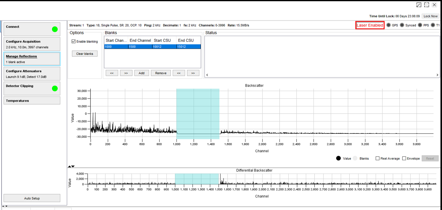
Figure 28: Created Blanking Zone
There is a requirement to see if the blanking zone has been added, if you navigate to the Surveillance Waterfall window you will see further evidence that the blanking zone has been created (Figure 29).
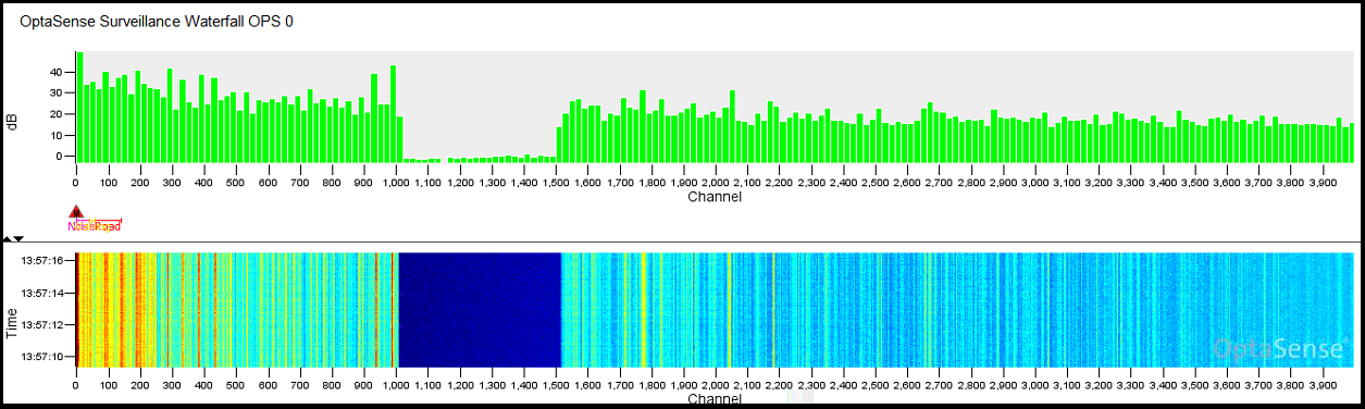
Figure 29: Surveillance Waterfall
Multiple Blanking Zones
The software has the ability to add multiple blanking zones. The process is the same as that for adding a single zone. Pressing the Add button will create a new blank in the table where the start and end channels need to be set. In Figure 30, you can see that there have been 3 blanking zones added.
Every time a new zone is added, it will be highlight light blue in shade, to identify that it has been added.
If there is a requirement to change the channel span, select the blank to be changed in the Blanks panel. The currently selected blank will be highlighted in blue. The shaded region on the backscatter will also be highlighted in light blue. Double clicking the Start or End cells allows these values to be adjusted as necessary.
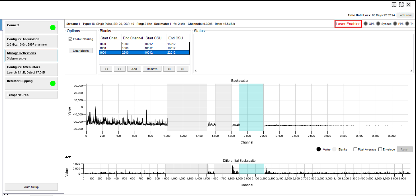
Figure 30: Multiple Blanking Zones
Removing Blanking Zones
To remove a blank, select the blank to be removed in the Blanks table and press the Remove button (Figure 31). It is also possible to clear all blanks by pressing the Clear blanks button (Figure 32).
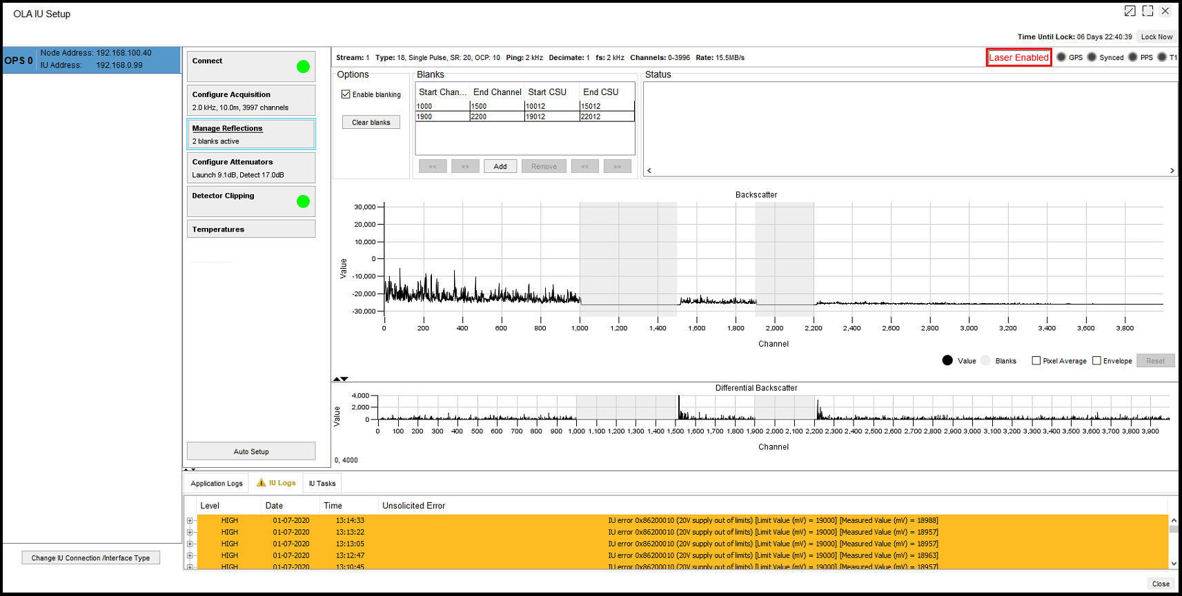
Figure 31: Blanking Zone Removal (Single)
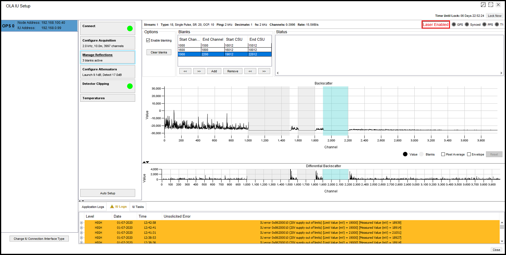
Figure 32: Clear all blanks
Using Blanking for Fiber Breaks
On occasions there may be a need to repair a fiber optic cable (FOC). There are several options to carry out this repair, but the main focus is to make sure that there is no damage to the Interrogator unit (IU).
If a fiber break alerts on the system, the operator needs to check the current and historic waterfall data to verify the loss of signal, where the signal has been lost and when it occurred. A fiber break (or significant attenuation event) will create a dead zone on the waterfall display. IU Setup can also help to identify the channel that a fibre break has occurred on.
IU Setup requires super-user access
Identifying a Fiber Break
When a fiber is broken it will be noticeable on the Surveillance Waterfall. The display will show a complete absence of signal from the point of the break to the end of the fiber. This will be followed by a Fiber Break alert appearing on the map screen with associated alert in the tote. The immediate action on a fiber break is to check the extent of the reflection caused in the IU Setup panel. Any reflection of concern will be at the point of the break and will be shown as a large spike above the usual backscatter signal.
The system will continue to operate as normal up to the fiber break but follow-on action must be taken to protect the IU from potential damage caused by reflected light.
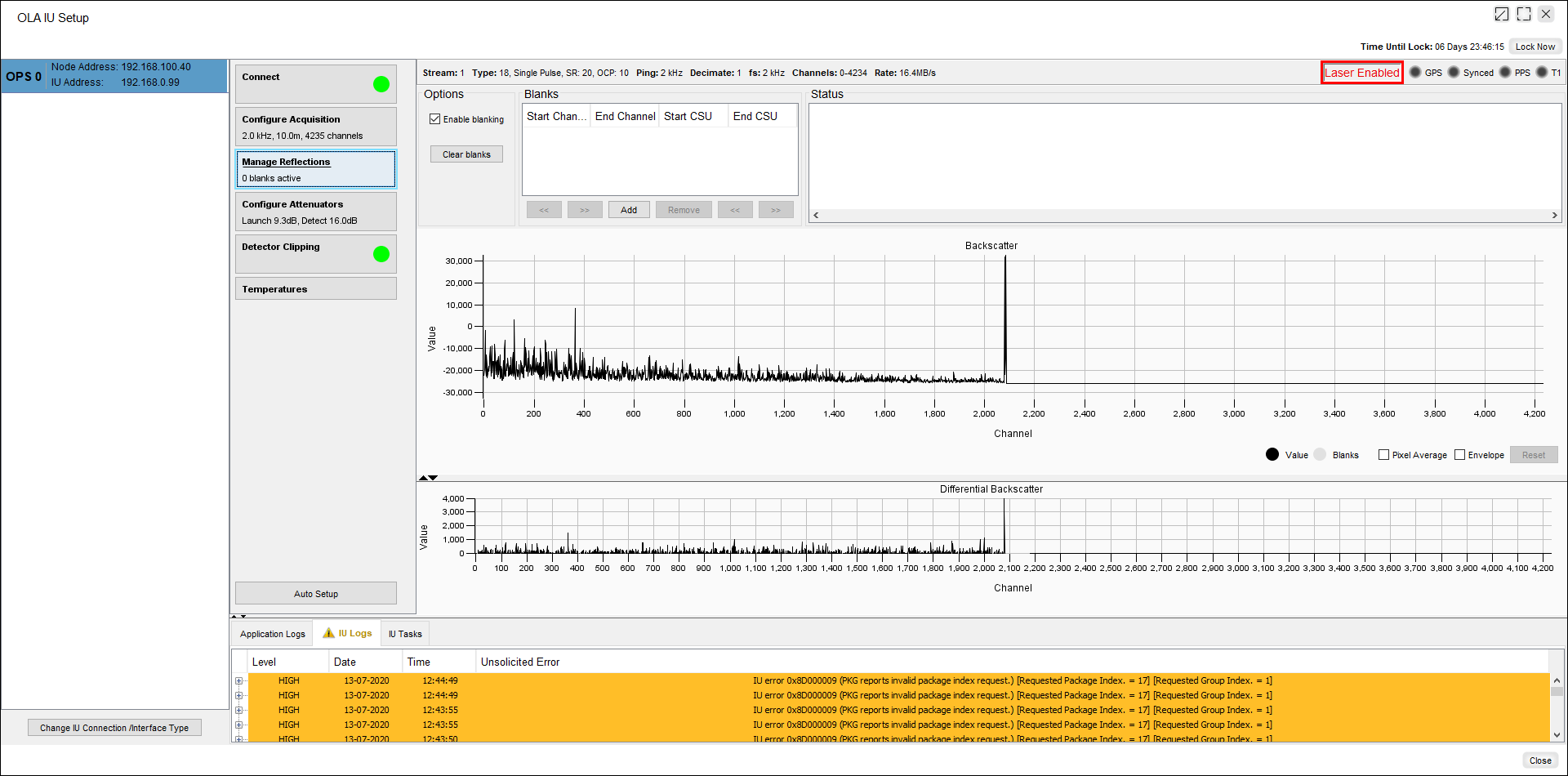
Figure 33: Reflection visible on the backscatter trace at channel 2080
Once a reflection has been identified then a ‘Blank’ can be added to protect the IU from reflection thus allowing the IU to be left operational until the fiber is repaired. The IU must not be left running in this state indefinitely.
Advanced Activities
Manual Attenuation in an OLA2.1(+)
Prior to setting the attenuators of the IU (using the Auto Setup function) the Interrogator must be placed into a SAFE mode to avoid damage. To do this, select the Configure Attenuators and set the Launch and Detect attenuators to approximately 30 dB. These values put the launch and detect stages into a safe state for initial power up and configuration.
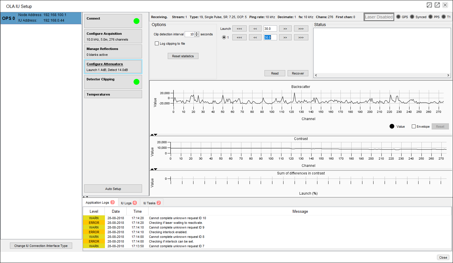
Figure 34: Configure Attenuators Display
To increase the Launch and Detect attenuators use the ‘>>’ buttons to increase the attenuation. The ‘>>>’ icon will increase attenuation by a greater amount. The ‘<<<’ and ‘<<’ buttons will reduce the amount of attenuation. It is also possible to type a value into the central box as press Enter to enact the change. The actual attenuation value may change slightly from the specified value once the system has made the change.

Figure 35: Launch & Detect Attenuation buttons
Once the attenuators have both been set to a SAFE state and the fiber has been checked with an OTDR to confirm no significant reflections are present then the laser can be switched on at the IU.
The aim in configuring the attenuators is two-fold:
- To set the launch attenuator to maximise the amount of the light launched into the fiber without causing non-linear behaviour in the fiber. Nonlinear behaviours is only likely to be evident in longer fibers (>10 km)
- To maximise to maximise the amount of light being detected without saturating the detector.
The skill involved is in identifying the point of non-linear behaviour, which we will cover in more detail in Section 8.1.2.
Observe the backscatter graph on the Configure Attenuators tab (Figure 36). The trace should appear fairly flat.
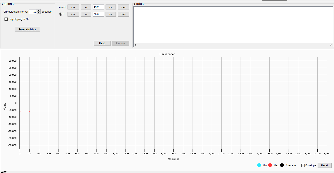
Figure 36: Launch attenuator SAFE, detect attenuator SAFE
Verifying reflection free conditions
In the first phase we will gradually allow more light into the system by reducing the launch attenuator in steps using the ‘<<’ button. What we are aiming to see is that no large reflections appear that are much greater than the average signal strength. You may need to zoom in on the vertical axis in order to see any signal.
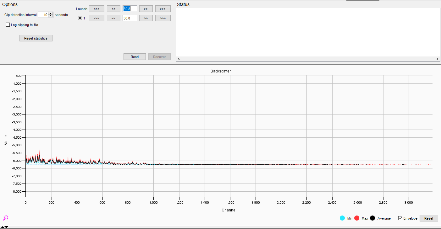
Figure 37: Launch attenuator position 30%
The detect attenuator is less important here - we are more concerned with how much light we are putting into the fiber at this stage.
If you are unsure about some data (whether it is structure or reflection) zoom in our further decrease the launch attenuator – it won’t cause any harm. What we are looking for are massive signals that may damage the detector. If any massive signal spikes are observed then the fibre should be repaired if possible and blanks implemented if necessary.
Detecting the point of non-linearity
As the launch attenuation is reduced, we are increasing the amount of light in the fibre and would naturally expect the detected backscatter level to also increase. However, once we have reached the point of non-linearity then the detected signal level will begin to drop. The launch attenuation setting where non-linearity is observed represents the optimum amount of light that can be launched into the fiber. We can observe the point of non-linearity by looking at the behaviour of the channels at the end of the fiber. We must do this at the end of the fiber as the non-linearity process is a cumulative process.
Zoom in on the last 200 channels. You won’t see much – just a vibrating trace (Figure 38):
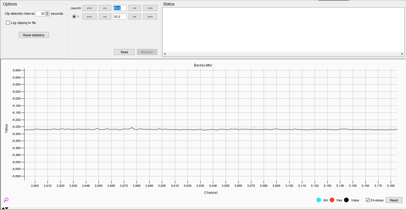
Figure 38: Not much signal variation in the last 200 channels.
As we start to reduce the amount of launch attenuation, we are going to see more signal appearing (Figure 39).
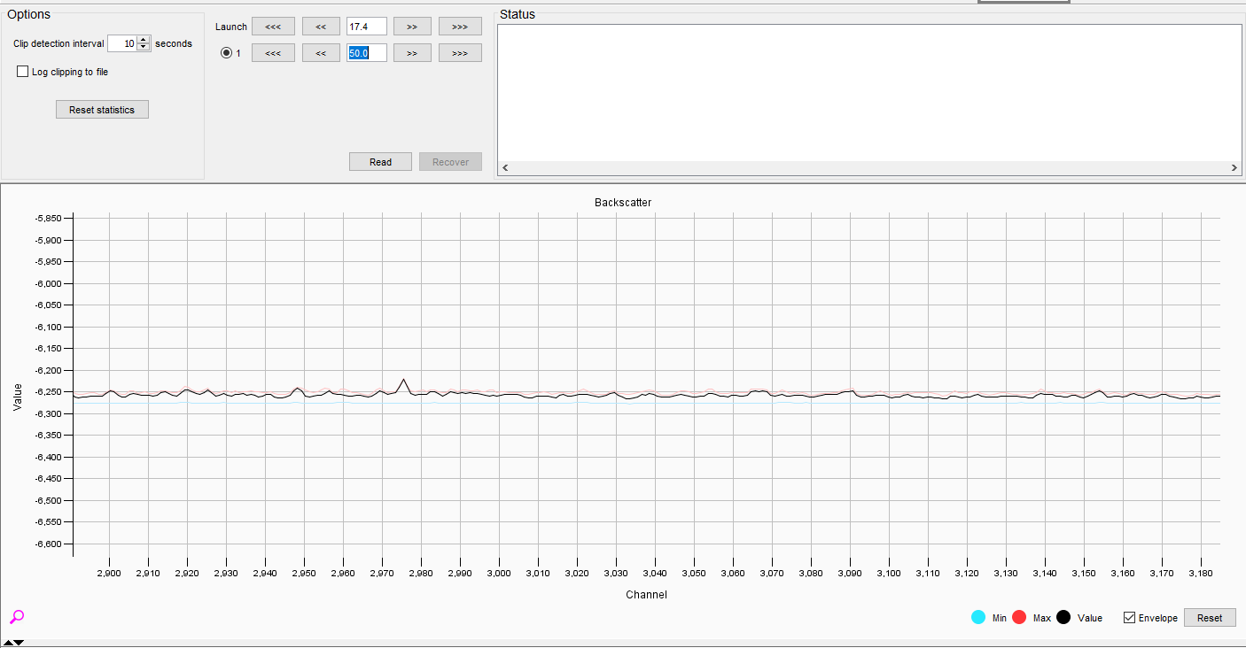
Figure 39: More signal appearing - here the max capture envelope (red) can be helpful
We have a problem though – there is not enough light in the detector to really capture what is going on. Reduce the amount of detect attenuation a bit to allow more light to be captured. There is a note of caution here: if the detect attenuation is reduced too far as well as the launch attenuation (which is what we will be doing to find locate the point of non-linearity) there is a danger of clipping. The system can tolerate some clipping but should not be left in such a state for extended periods. As you are reducing the launch attenuation, keep an eye on the clipping traffic light and occasionally take a look at the whole trace backscatter trace. Keep in mind that as more light is launched into the system we can raise the detect attenuation level in order to prevent clipping and keep the detector safe. Remember, all that we do with the detect attenuation is scale the signal up and down – what we are more concerned about is finding the optimal launch condition.
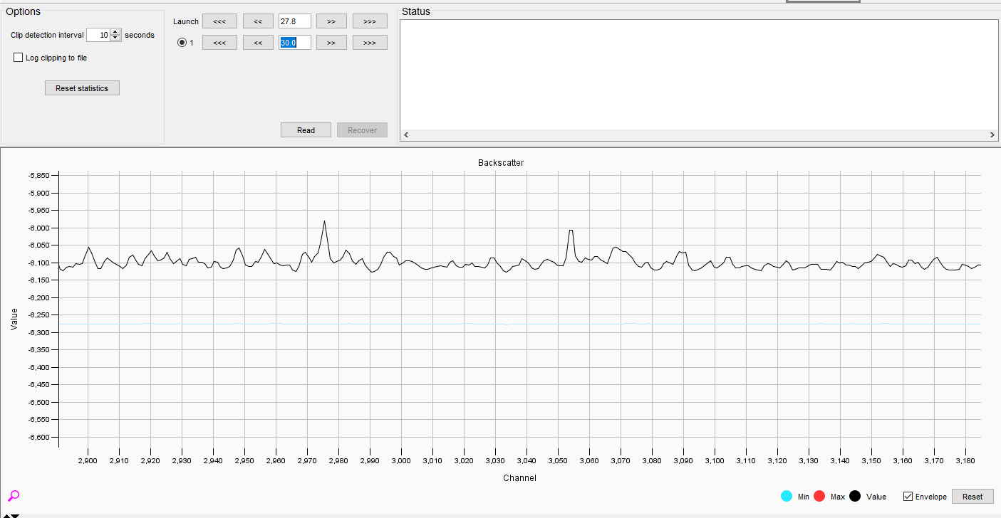
Figure 40: Opening up the detect attenuator lets in more light and we can see structure in the signal
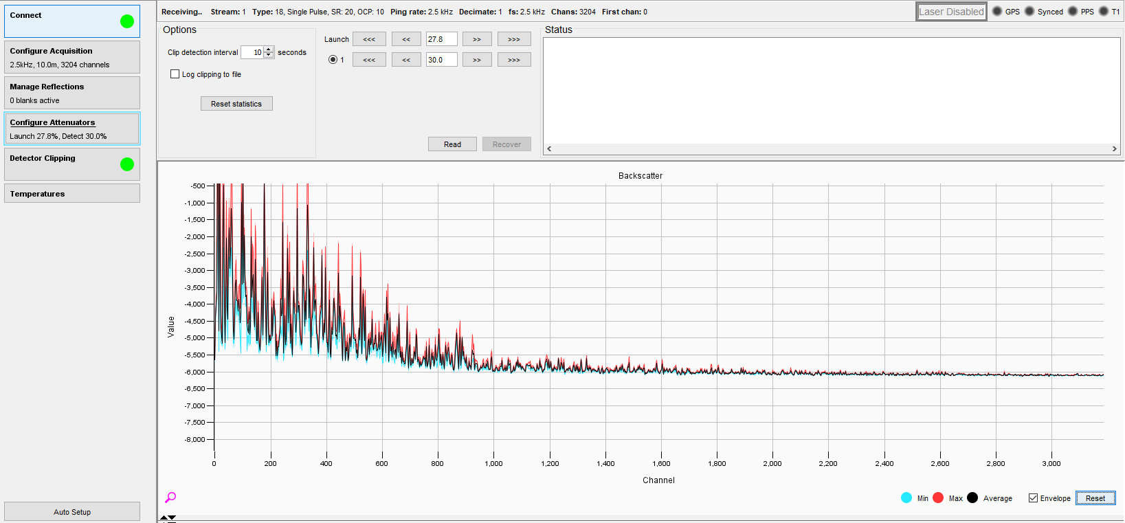
Figure 41: The overall trace. Keep an eye on the envelopes and the detector clipping light
In the series of figures shown below (Figure 42 to Figure 44), watch the signal trace rise as the launch attenuation is reduced.
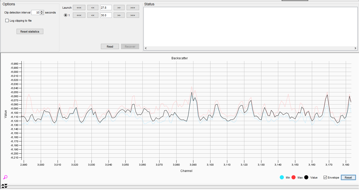
Figure 42: Launch Value of 27.8
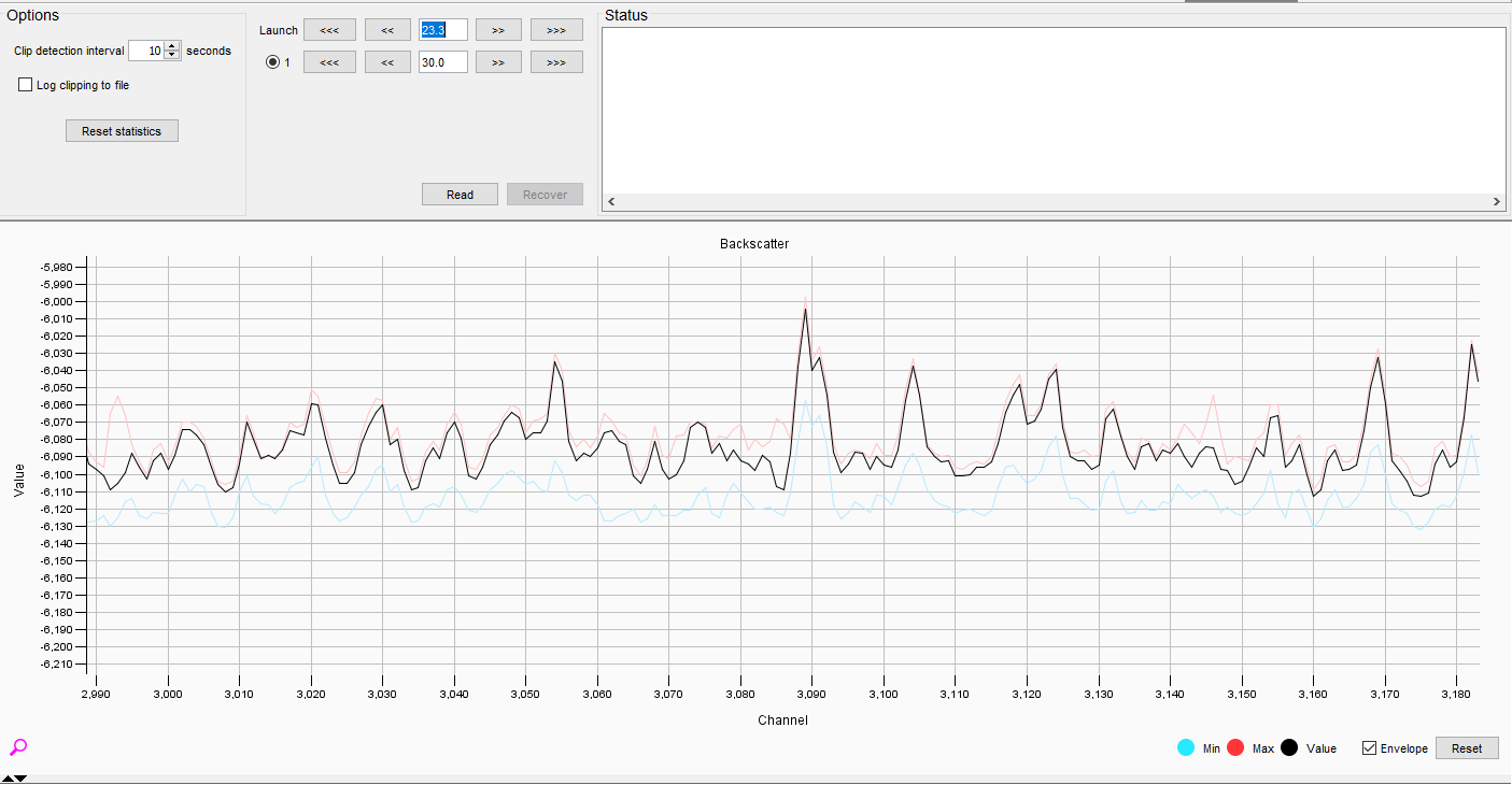
Figure 43: Launch Value of 23.3
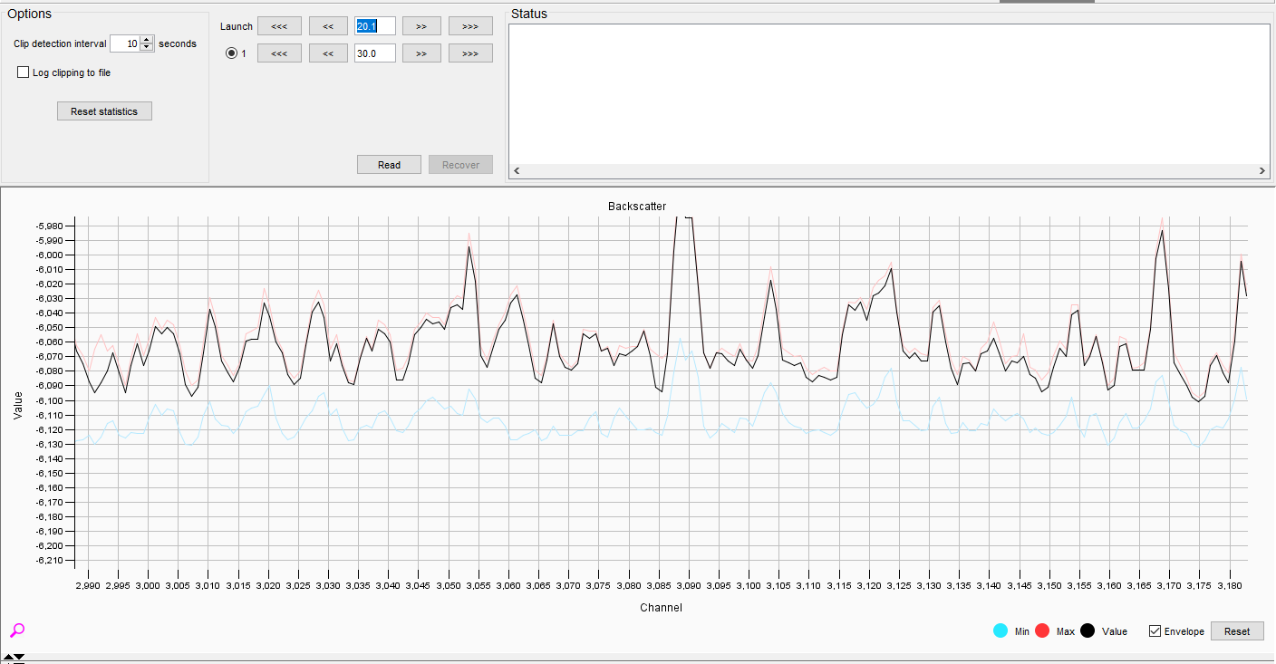
Figure 44: Launch Value of 20.1
Eventually a point is reached where launching more light into the fiber causes the amount of light at the end to actually drop – this is the key point of interest. As we are looking for this keep a very close eye on the clipping situation – it’s OK to increase the detect attenuation in order to prevent clipping. The detect attenuation only scales the signal, it doesn’t change it.
Setting the Launch Attenuator
Having found the optimum launch condition for the fibre, we don’t leave it at this point. Remember fading. We know that fading affects the gain in the channels and so if we left the launch attenuation at the maximum it would be expected that some channels we are looking at will be faded and when not faded they may enter into non-linearity.
We therefore want to increase the launch attenuation a little to allow for this effect. A recommended increase is to make 5 small step (‘>>’) increases.
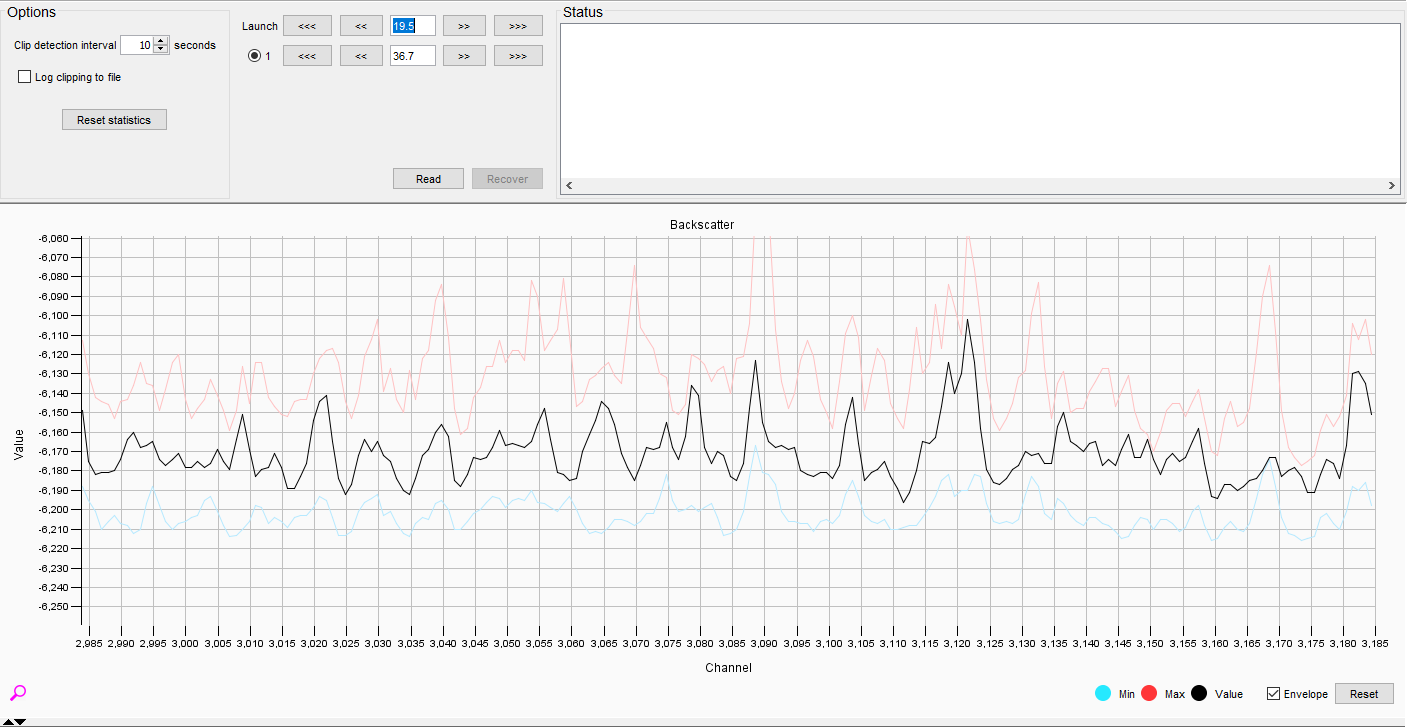
Figure 45: Final Launch Setting
Setting the Detect Attenuator
We are now finished with launch and can set the detect attenuation level. Reset the display and zoom into the first 1,000 channels.
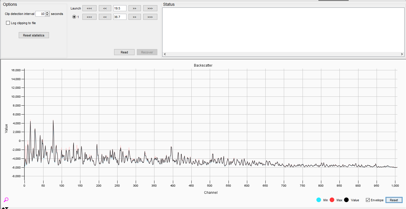
Figure 46: In the full trace it is clear we have some clipping
Clipping occurs when a channel is saturated and further decreases in the detect attenuation cause “flat topping” of the peaks. This effect can be seen by comparing Figure 47 and Figure 48.
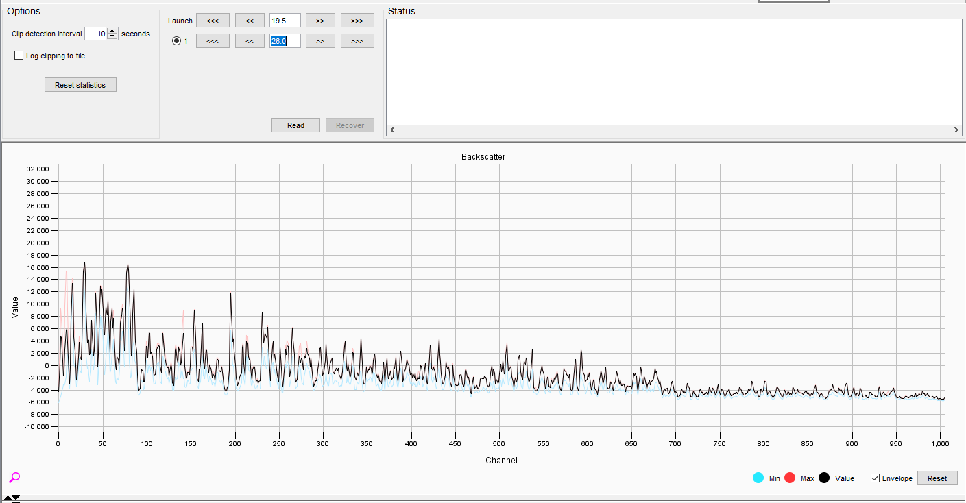
Figure 47: Point Before Clipping Occurs
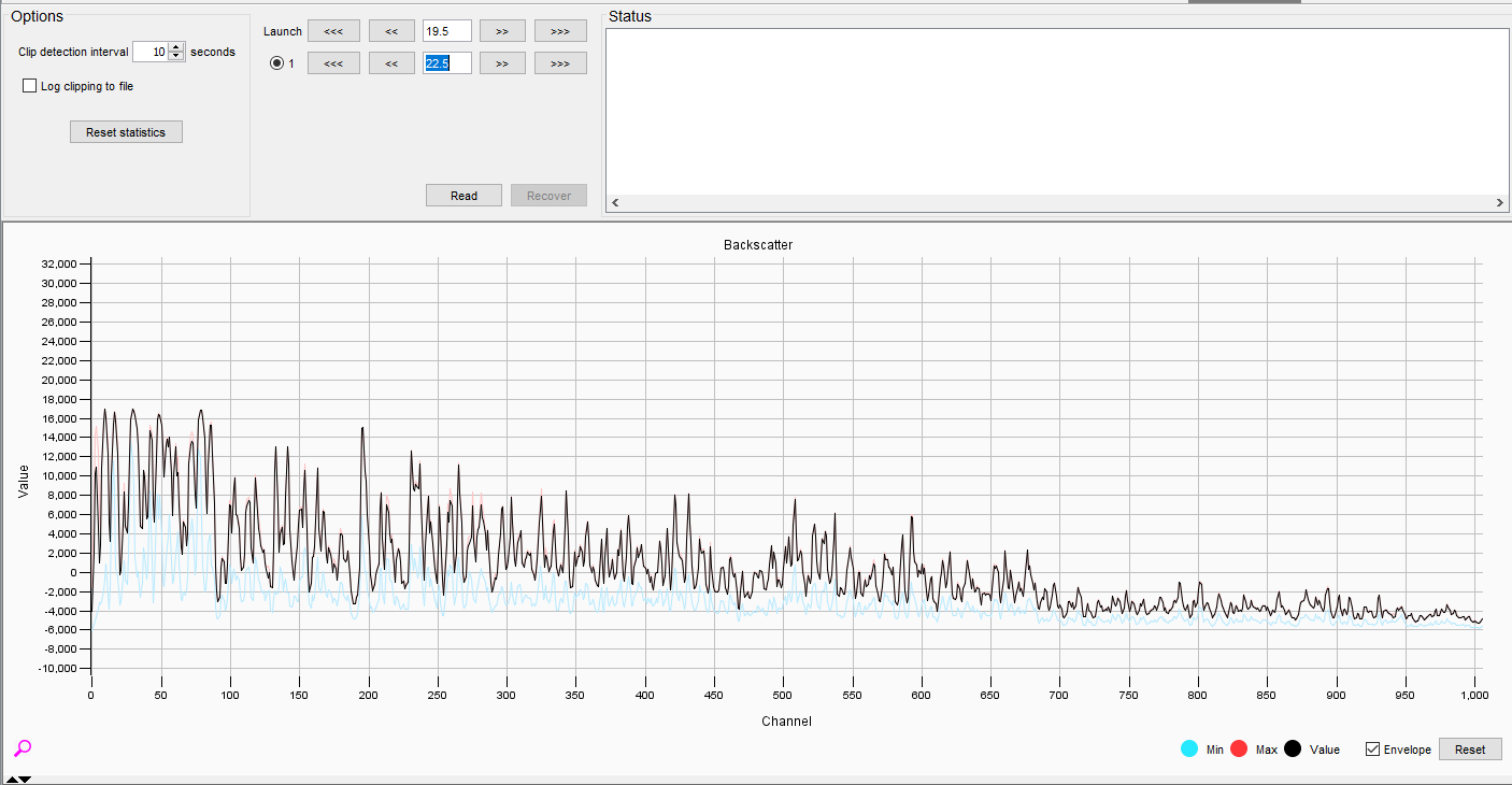
Figure 48: We can see the peaks near the front of the system are becoming flat and round at the top
Zoom in and increase the detect attenuation until there is daylight between the actual trace (black) and the maximum enevelope (red).
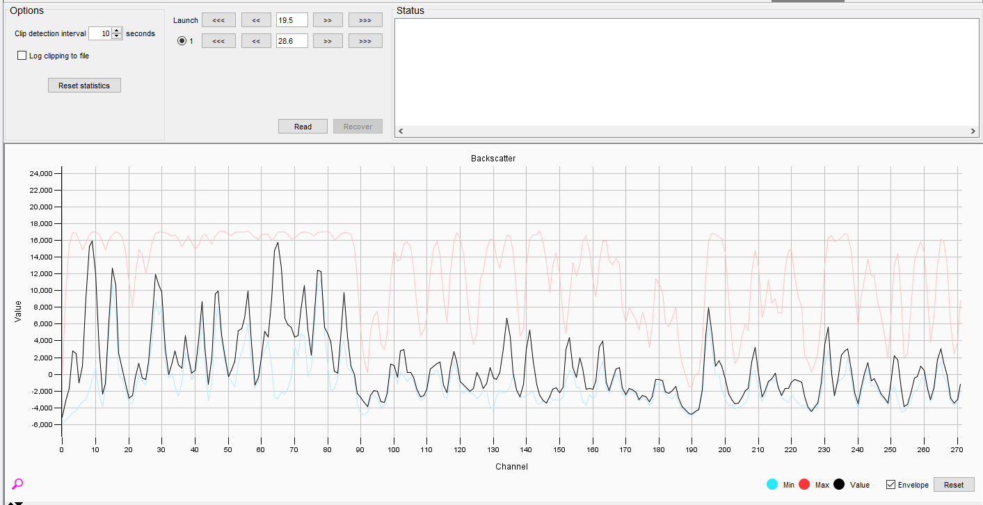
Figure 49: No clipping point located
Again, to account for fading we can increase the attenuation a little further. This is less of a concern than on the launch attenuator. On the detect attenuator some clipping is to be expected in a well-tuned system.
Manual Attenuation in a QuantX
Setting the IU into a safe condition before turning on the laser
The interrogator is fitted with two attenuators which act to adjust light levels in the system:
- Launch attenuator – adjusts the amount of launched light. Can be used to limit the light launched into a long fiber and ensure that operations are within the linear regime
- Detect attenuator – used to adjust the received light level to ensure it is not limiting or clipping at the detector.
Prior to setting the attenuators for the IU, the Interrogator should be placed into a high attention setting. This is achieved by increasing the Launch and Detect attenuators (or by typing the required attenuation into each box and hit enter). Set the Launch to 20dB and the Detect to 40dB.
First, READ the attenuators by pressing the button – this will then populate the attenuator settings:
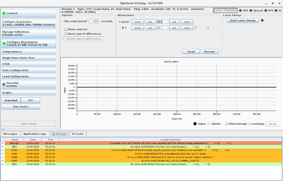
Figure 50: Configure Attenuators Display
In order to visualise the backscatter trace, the acquisition mode Data Type should be set to Scope Mode with the appropriate number of carriers for the intended mode of operation**.**
Once the attenuators have both been adjusted to a safe setting, and the fiber has been checked using an OTDR to confirm no large reflections, the laser can be switched on by setting both key-switches to the ON position. [See the IU Manual for more details].
The status bar in IU Setup will show when the laser is enabled/disabled.
After turning on the laser, allow a few minutes for the laser to stabilise before making adjustments.
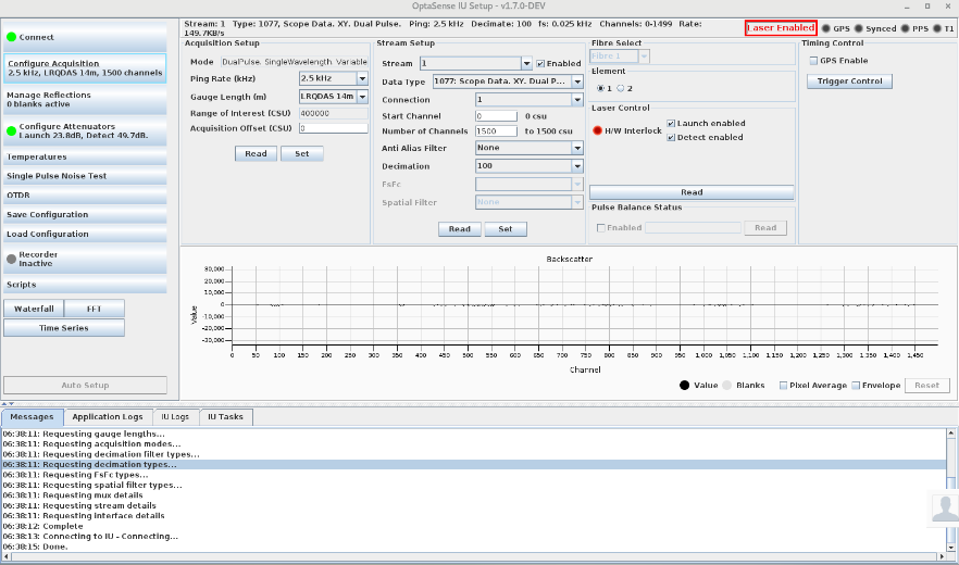
Figure 51: Configure Acquisition Display
The backscatter displays are used for setting up the unit and will be blank when phase data is selected. For data types where more than one sample value per channel is available, the Element buttons select which value is displayed. The Element buttons appear only on the configure acquisition screen and should be moved-between when configuring the attenuators.
To zoom, click and drag with the left mouse button. When zoomed-in, a magnifying glass is shown in the bottom left of the display. Click the right mouse button to zoom out again.
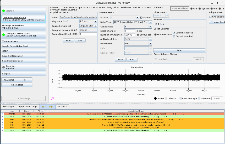
Figure 52: Zoomed in to see some backscatter
The envelope option plots the minimum and maximum value envelope of the series, until reset by clicking the “Reset” button.
The pixel average option provides an alternative view of the data when there are many more channels than horizontal pixels. When selected, this plots the average value at each pixel position, as well as the minimum and maximum at that pixel.
Optimising the Attenuators
Identify the end of the fiber
Using scope data to view the backscatter, select the Configure Attenuators tab. Reduce the launch and detect levels until the backscatter is visible and you can identify the end of the fiber (Figure 53):
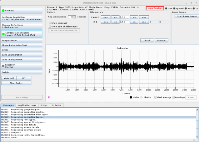
Figure 53: Identifying the end of fiber
The x-axis is presented as scope data where each sample is 1ns long (approx. 0.1m)– this is different from the output of the device, as detailed in the data sheet which refer to phase data which can be selected to be output as 10ns – approx. 1m or 100ns – approx. 10m.
Setting the Launch Power
The objective when setting the launch power is to maximise the power under the constraint of “linear behaviour” �– if we inject too much power into the fiber, the signal will go non-linear at some distance down the fiber – the lower the power, the further out that point is. Our aim is to maximise the amount of power going into the fiber, while ensuring that the last set of channels monitored are behaving linearly (with a safety gap).
To do this, gradually decrease the launch attenuator until you can see the onset of non-linearity. The correct behaviour as we reduce the attenuation (increase power levels), is for the amplitude of the backscatter pattern at the end of the fiber to increase. At the non-linear point, the trace will change and become distorted. You may find the pixel average and/or envelope buttons useful here to identify the range of values. Also, just zoom in on the top half, it’s symmetric. Once the non-linear point has been identify it is sensible to increase the launch attenuation a little further.
Zooming in on the last few thousand channels is often easier. Values can be entered directly into the boxes in order to change attenuation with more or less finesse (the value entered may not coincide with a valid setting and the final position may differ slightly).
Adjust Detect Attenuator
Zooming back out, the detect attenuation can now be optimised. The aim here is to control the level of light coming back into the detector – again we want to maximise our signal. All that is needed is to reduce the detect attenuator until the display is maximised with no clipping. Do not touch the launch attenuation once it has been optimised.
Note: you may find in certain pairings of Launch Attenuator and cable that you can reduce the detect attenuator to zero without observing clipping – this is not a problem.
The clipping behaviour is shown below. What you will find is that clipping will be observed from the front outwards. This is undesirable and the detect attenuator needs to be reduced to the point where no clipping is observed.
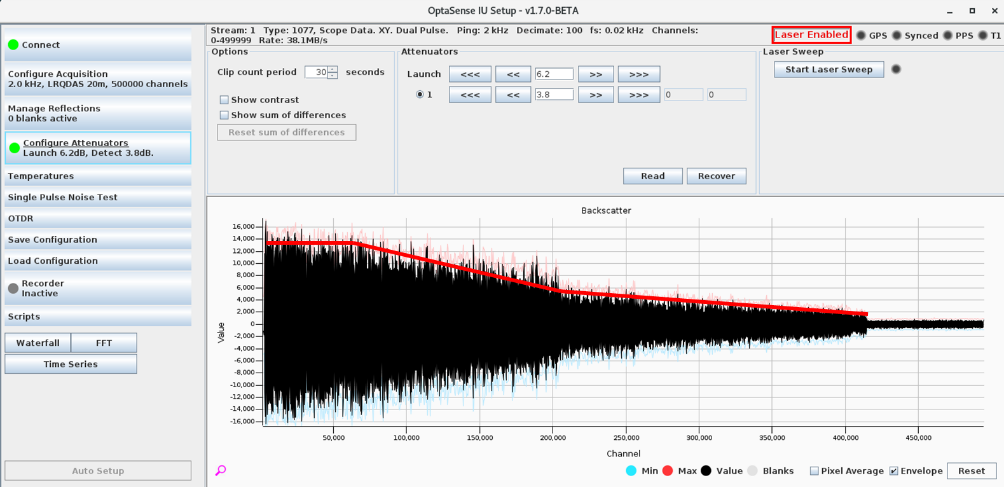
Figure 54: Detector clipping highlighted at the front end of the fiber
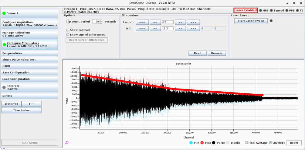
Figure 55: Corrected behaviour (bottom)
Confirming behaviour for element 2
If the intended final configuration is to use dual carriers then once this process has been completed for the first element it also needs to be checked for the second, we can go back to the Configure Acquisition panel, select Element 2 and then confirm that it also is not in a non-linear launch state or clipping at the detector.
Leaving “scope mode”
Once this process has been completed, we can go back to the Configure Acquisition panel and select the appropriate Data Type for the final configuration. When acquiring Phase Data**,** the Configure Attenuators panel will not display a backscatter trace. At this point, you could reduce the number of acquired channels to those that you will use.
Verifying the first acquisition point
To do this we need to zoom into the first few channels of the fiber coverage to assess the signal that is being received.
From the histogram (Figure 56) we can see that there is a low-level signal until about
channel 9.
This suggests that the system is acquiring too early – this has some implications:
- The location of the TRUE optical distance will be shifted accordingly down the fiber.
- We will miss useful information at the beginning and the end of the sensing fiber.
We can test that the system is acquiring too early or too late by creating some artificial noise, through tapping the fiber 1 m away from the box. We see the difference between the stimulated and
non-stimulated section of fiber confirming that the location of the fiber 1 m from the box is actually being reported at a distance of some 110 m (11 channels in this fiber setup).
As well as correctly configuring the IU we can also use this process to account for other discrepancies such as patch cables or lead-in cables. If the start location needs to be moved, please contact OptaSense for remote assistance.
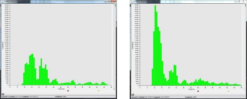
Figure 56: No stimulation (left) and tapping fiber 1 m away from the IU (right)
Masking a noisy environment at the start of the fiber
An IU can be located in varying environments; it may be housed in a remote valve station in a sparsely populated desert or may be housed in a building located in the middle of a vast industrial refinery area. For this reason, several channels at the start of the fiber may wish to be masked out as they are very noisy and in a secure area; they could distract from what the operators are looking for. It may be required that the installer sets the first acquisition point to be the first channel outside the industrial site.
In order to do this, it is important to find exactly where the extremity of the industrial area is located by sending someone out to geo-reference and accurately locate how many channels need to be masked.
If we have 110 metres of fiber located in a noise industrial site which the customer would like us to mask out, we must alter the first acquisition point field located in the Configure Acquisition tab within the IU Setup window for the OPS you wish to set. For this example, the first acquisition point should be set to Channel 11. This is due to the spatial resolution set at the default setting of 10 metres.
Once a new first acquisition point has been entered the Set button needs to be toggled.
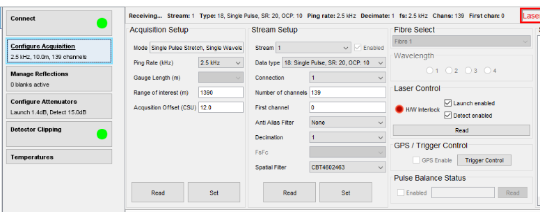
Figure 57: Altering the first acquisition channel
Fiber Assurance Stream
Previous versions of software have required the configuration of a fiber break detector in order to provide the ability to detect if and where a fiber break had occurred. Any version of software running IU setup 1.8 or greater contains a self-configuring fiber assurance stream (available on OLA2.1+, OLA2.2 and QuantX at present). The assurance stream should be enabled once the IU has been fully configured by checking the ‘Enable processing’ box on the IU Processing tab in IU setup (Figure 58).
Once checked, the IU data stream will drop out for several seconds whilst the fiber assurance stream is set up. After this point, the processing will automatically generate an alert should a loss of signal be detected anywhere along the fiber route (Figure 59). Once a fiber break has been detected the fiber assurance stream will need to be enabled again once remedial works have taken place.
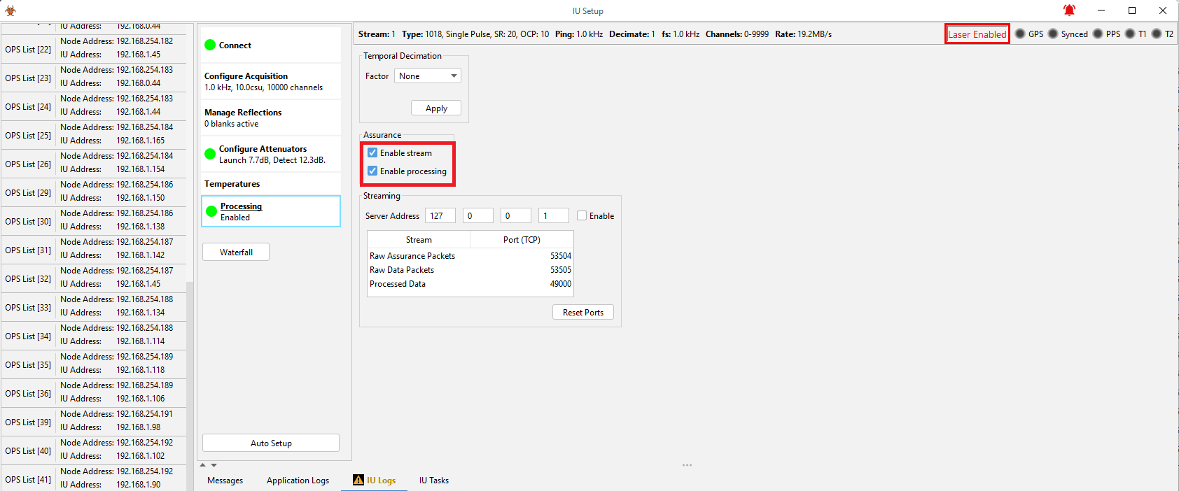
Figure 58: IU Setup showing where to enable the fiber assurance processing
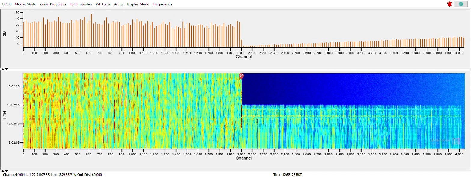
Figure 59: Waterfall showing a loss of fiber signal and subsequent alert
Temporal Decimation
In some scenarios it may be desirable to reduce the data sampling rate without reducing the IU ping rate. For example, on a quantitative system a higher ping rate improves the strain rate that can be tracked while we may only be interested in very low frequency signals. A reduction in the data rate can be achieved by applying temporal decimation, which can be configured on the ‘Processing’ tab of IU Setup. The appropriate decimation factor should be selected and then applied. Once applied, the icon on the 'Processing' tab will turn green and the stream parameters will list the decimation factor and reduced sampling rate (Figure 60). On an ODH-F IU operating in a quantitative data mode there should always be a temporal decimation factor of at least 4 applied owing to the way in which these systems determine phase.
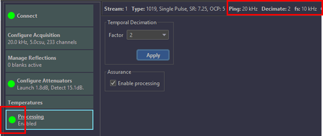
Figure 60: IU Setup with a temporal decimation factor of 2 applied